3 Data Preparation
This chapter demonstrates how to process and prepare input data for Digital Soil Mapping (DSM) using the statistical software R. The processing steps are illustrated with a sample dataset. The chapter is divided into three parts:
Section 3.2 Point data preparation: Loading and processing a point dataset.
Section 3.3 Covariates preparation: Loading and processing a stack of gridded covariate (GIS) layers.
Section 3.4 Regression matrix: Creating a regression matrix, which is a data object used as input to fit a statistical DSM model.
Note These parts from a data preparation ‘workflow’ that should be run in sequence. The output objects generated in Part 1 and Part 2 are used as input for Part 3.
After completing this tutorial you will be able to:
- Load data tables and GIS raster (GeoTiff) files in R.
- Perform common data processing steps.
- Convert tabular objects to spatial data (and vice versa).
- Mask and project a covariate stack.
- Extract raster values at data point locations.
- Create a regression matrix.
3.1 Set up
The required R packages for this chapter are:
- dplyr: A grammar for data manipulation.
- sf: Handling vector (point, line and polygon) data.
- ggplot2: A system for creating elegant data visualizations using the Grammar of Graphics.
- terra: Spatial data analysis
- caret: Classification and regression training
At the beginning of each section, the necessary packages will be specified. If a package is not installed, you can use the install.packages() function to download and install it.
# To check if a package is installed
system.file(package = 'terra')

# it prints the directory where the package is installed
# otherwise, an empty directory is printed as ''

# To install a package uncomment (i.e., remove the '#') the following line
#install.packages('terra')
The input data for the tutorial is available on the ISRIC WebDAV. We will retrieve the data directly from the URL using R functions. The WebDAV is organised into folders, similar to the structure on your local machine.
It is considered good practice to avoid hard-coding file paths, file names and variable names in your code. Instead, store these R objects, which can then be reused throughout the code. This makes your code more versatile and easier to adapt.
Indicate the working directory on your local machine. Additionally, define an object that stores the output data directory (folder). Note that this directory must already exist within the working directory, as the code below will not create it.
Next, we define some variables to make the code reusable. All of this information is derived from our input data. In this step, we specify the variable and region of interest. The paste() function is used to combine the various components of the output file.
As mentioned in Chunk 3, our target variable for mapping in this tutorial is Soil Organic Carbon content (SOC (%)) in Ghana. This variable is stored in column called orgc in our points dataset.
The following global option will prevent very large numbers, such as coordinates in projected systems, from being printed in scientific notation.
# to avoid scientific notation
options(scipen=999)
3.2 Point data preparation
This section shows how to load a soil point dataset into R and perform several processing steps to prepare the data for digital soil mapping. These steps include:
- Section 3.2.1: Loading a soil point dataset in
R - Section 3.2.2: Data exploration: soil properties
- Section 3.2.4: Data exploration: spatial
We will need the following libraries in this section:
# load libraries
library(dplyr)
library(sf)
library(ggplot2)
We now define the objects that contain the file path to the input data, as well as the file path with the GIS file that contains the boundary of the study are, which will be used for plotting later. These paths were defined in Chunk 1. Note that the input files are located in sub-folders within the input data folder. We use the function file.path() to construct a full file path by combining the input data folder, the sub-folder and the file name.
# load points table
pointsFile <- file.path(url, PointsFileName)

# file path of GIS file with study area admin
adminLayerFile <- file.path(url, adminLayerFileName)
Similarly, we define the name and location of the output files created by this script, as shown in Chunk 2. In this case, we will create an R output file in rds file format. This file will contain the processed soil point dataset and will be stored in a folder named output within the working directory.
# output location and name of the file that stores the processed point data
pointDataFile <- file.path(outputDir, "pointData.rds")
Finally we check the coordinate system of the points, defined in Chunk 4, which is the WGS 84. The EPSG code for this projection is 4326.
3.2.1 Loading the soil point dataset
We start by reading the points table using the read.csv() function and inspecting its contents. To do this, we will use the str() and head() functions.
# read the soil data
d <- read.csv(pointsFile)
# inspect data
str(d)# also try
head(d)3.2.2 Data exploration: soil properties
Before starting the modelling process with the dataset, it is good practice to first explore the data to ensure that the measured values fall within expected ranges. We can explore the data by calculating summary statistics and plotting histograms. Examples are provided below.
# calculate summary statistics
summary(d[variable])
Pay special attention to the minimum (0.22) and maximum (3.42) values of the selected variable SOC. Analyze whether these values fall within the expected range.
Next, we will plot a histogram and a boxplot for the variable SOC.
# plot histogram
hist(d[[variable]],
     col = "lightblue",
     xlab = xlab,
     main = main)
rug(d[[variable]])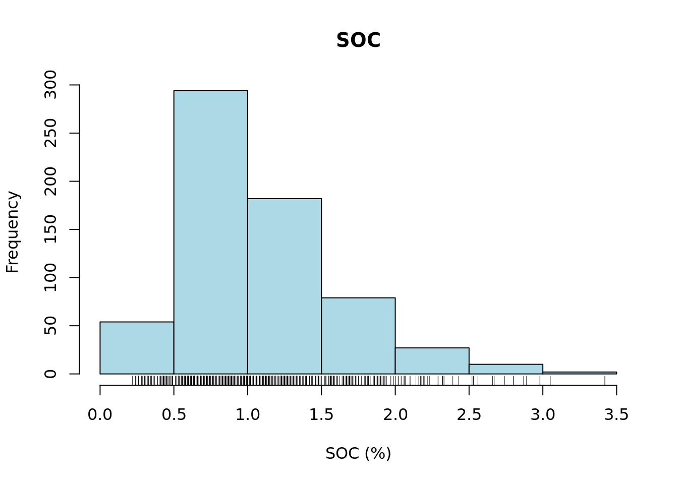
# plot boxplot
bxplt <- boxplot(d[[variable]],
                 col = "lightblue",
                 xlab = xlab,
                 main = main)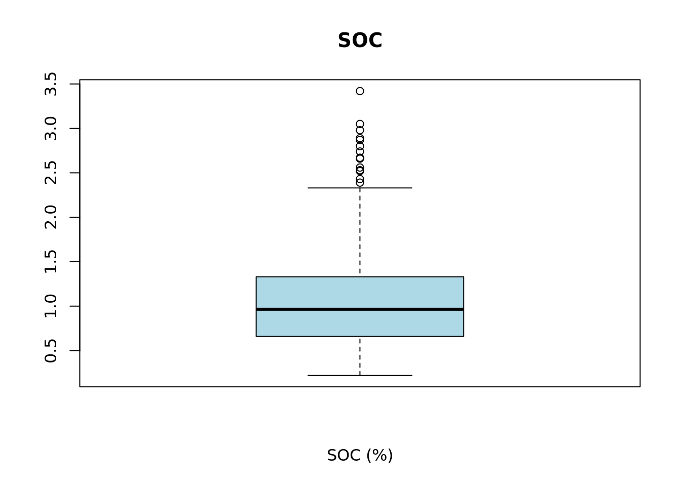
We can inspect the elements that make up the boxplot by saving it to a variable, in this case bxplt, and then printing its contents.
bxpltThe fifth element of the stats vector inside bxplt contains the value of the upper whisker.
# extract upper whisker value
upper_whisker <- bxplt$stats[5]

# check value
upper_whisker
[1] 2.33From the summary statistics, histogram and boxplot we can see that the data distribution is left skewed and that there are only few layers with SOC larger than the upper whisker of the boxplot 2.33%. Let’s check now the number of layers.
# plot histogram
sum(d[variable] > upper_whisker)
[1] 14Indeed, there are only 14 observations out of 648 that are higher than 2.33%. Although these are a valid values, we assume for the sake of this exercise that these are “outliers”, and we filter them out of the dataset.
d <- subset(d, d[variable] < upper_whisker)Dealing with outliers must be done with caution. As a general rule of thumb, values that fall outside 1.5 times the inter-quartile range are considered outliers (these appear as single dots in the boxplot). However, this is just a convention, not a rule with a strong theoretical foundation. In general, one should be very careful when removing outliers. This should only be done if the values are known to be erroneous or if the observations do not belong to the population we wish to model and map.
3.2.3 Selecting target soil layers
The soil dataset contains both topsoil and subsoil layers. By definition, the topsoil corresponds to the 0-20 cm layer, and the subsoil to the 20-50 cm layer. These depth intervals are recorded in the upper_depth and lower_depth variables in the input soil dataset. However, in some cases, obstructions in the soil prevented reaching the target depth. The actual depth reached during sampling is recorded in the sample_depth variable.
Here we choose to map the SOC content for the 0 - 20 cm layer. Ideally, we would only select layers that were fully sampled across the entire depth interval. However, to avoid being to restrictive, we accept layers where the sampled thickness is at least 15 cm. For the purpose of this exercise, we consider these layers ‘representative enough’ for the target depth layer.
We now proceed to select all topsoil layers from the soil dataset that have a sampled depth greater than or equal to 15 cm.
Remember that we stored the depth information in objects at the beginning of this chapter in Chunk 3.
d20 <- subset(d, d["upper_depth"] == model_start_depth & d["sample_depth"] >= min_thickness) Next, we plot a histogram of the target soil property using the selected layers.
# plot histogram
hist(d20[[variable]],
     col = "lightblue",
     xlab = xlab,
     main = main)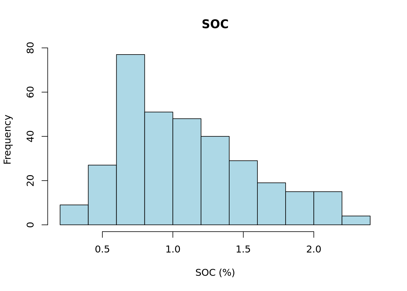
3.2.4 Data exploration: spatial
We continue our data exploration by creating a spatial point plot. To do this, we use the st_as_sf() function from the sf package to convert an R object—specifically a data.frame—into a spatial (sf) object. The column names containing the coordinates are passed to the coords argument. The crs argument is used to specify the coordinate reference system using an EPSG code. In this case, the soil sample data is in the WGS 84 [EPSG:4326] projection.
# convert to spatial object
d20_sf <- st_as_sf(d20, coords = c(lon, lat), crs = epsg_number_points)
# inspect object
str(d20_sf)You can see that the d20_sf object is now an sf (spatial) object. We can extract the geometry with the st_geometry() function.
# show at geometry information
st_geometry(d20_sf)
Geometry set for 334 features
Geometry type: POINT
Dimension: XY
Bounding box: xmin: -2.940605 ymin: 5.063508 xmax: 0.8880955 ymax: 11.03657
Geodetic CRS: WGS 84
First 5 geometries:Notice that the first line from the above output contains the number of points: Geometry set for 334 features.
To visualize the geometry of the dataset we can use the base plot() function, but a more polished and informative plot can be created with the ggplot package. We can also overlay the border of Ghana, which is stored as a GeoPackage file. This file can be read with the st_read() function of the sf package. Note that the projection of this administrative boundary file is WGS 84 [EPSG:4326].
# load admin file
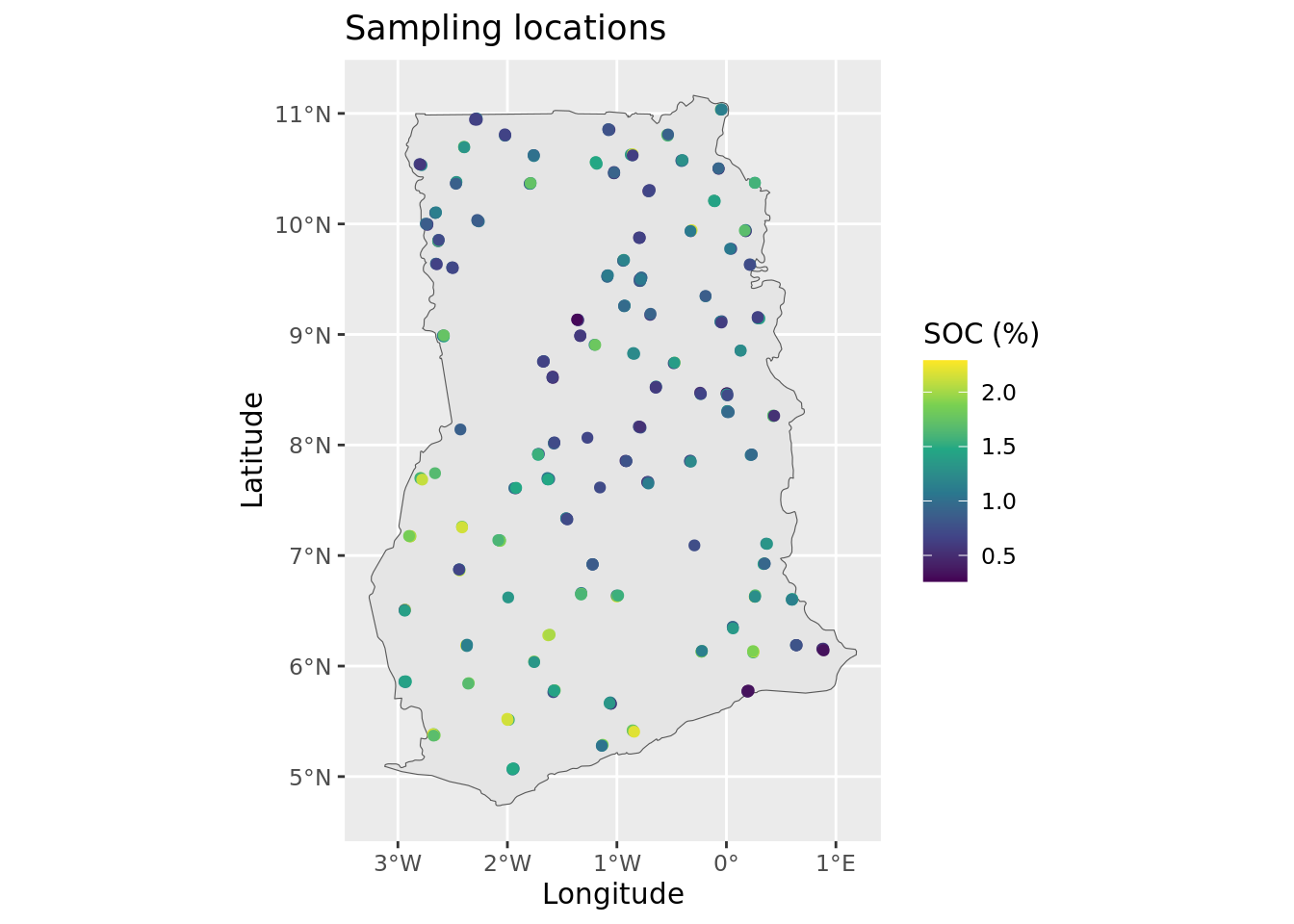
admin <- st_read(adminLayerFile)# plot map
ggplot() +
geom_sf(data = admin) +
geom_sf(data = d20_sf) +
ggtitle("Sampling locations") +
xlab("Longitude") +
ylab("Latitude")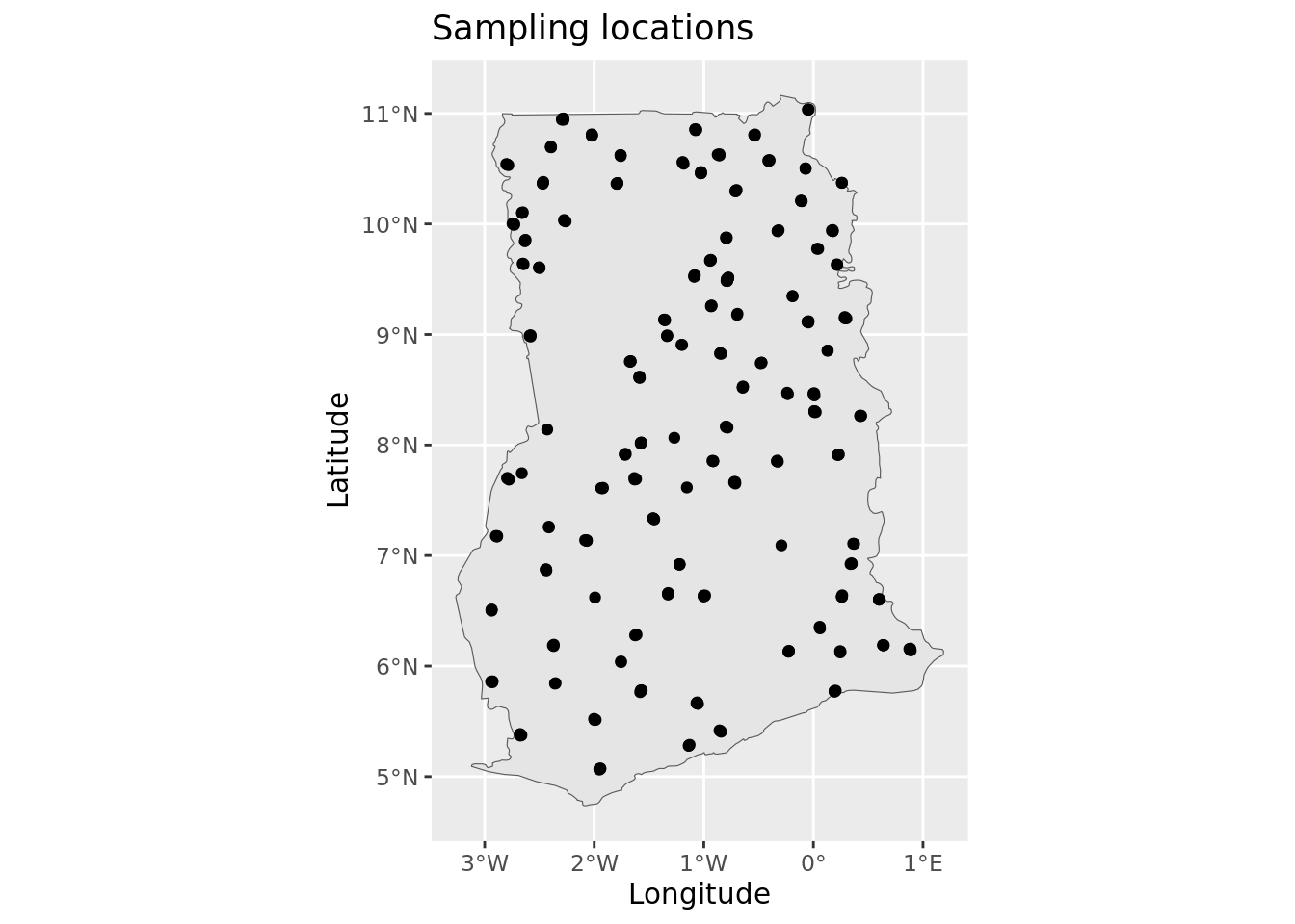
This plot confirms that there are no obvious issues with the georeferencing of the sampling sites—the points appear to be correctly located within the Ghana border. Note: ggplot automatically handles differences in coordinate reference systems, so even if the points and the boundary were in different projections, the plot still render correctly.
It is important to note that up to four plots were sampled at each of the location indicators shown on the map. The four plots are situated within a 2 x 2 km area and cannot be visualized individually because at this map scale.
We can further enhance the plot by visualizing the actual SOC values.
Now that we are finished, we save the processed dataset to the hard disk as an rds file. The .rds format is an alternative to .rda or .RDATA, with the key advantage that it compresses the data, resulting in significantly smaller file sizes on disk.
saveRDS(d20_sf, file = pointDataFile)3.3 Covariates preparation
This section shows how to load a covariate stack in R and perform several processing steps to prepare it for digital soil mapping. These steps include:
Section 3.3.1: Loading a set of GeoTIFF layers in R as a stack object
Section 3.3.2: Masking and exploring the covariate stack
Section 3.3.3: Selecting covariate selection through near-zero variance analysis
Section 3.3.4: Checking and cleaning the stack
This manual uses the covariates that where compiled for national-scale mapping. These covariates have global coverage at 100 m but were resampled at 1 km for this exercise. Layers for Ghana were clipped from the global 1 km stack using a rectangular bounding box.
We will need the following libraries in this section:
# load libraries
library(terra)
library(caret)
We now define the objects that store the file paths to the input data objects, specifically the covariates directory and the mask file. These paths were defined in Chunk 1. Note that the input files are located within sub-folders inside the main input data folder. To construct the full file path, we use the file.path() function, which combines the input data folder, the sub-folder and the file name.
# directory where covariates are stored
covarsDir <- file.path(url, covarsDirName)

# text file listing the file names of the covariates
covarsList <- file.path(covarsDir, covarsListFile)

# location of the mask file
maskFile <- file.path(url, maskFileName)
We now define the name and location of the output file(s) generated by this script, as shown in Chunk 2. In this case, we will create a single RDS output file. This file will contain the processed covariate stack in data.frame format and will be stored in a folder named output within the working directory.
# location and name of the file that will store the map object
covarStackFile <- file.path(outputDir, "covariateStack.rds")
Finally, we define an object that stores the coordinate reference system (CRS) of the data, as previously outlined in Chunk 4. The coordinate system of the covariates is the Interrupted Goode Homolosine. The EPSG code for this projection is Interrupted Goode Homolosine. The terra package can handle EPSG codes using the following notation: <authority>:<code>, which, in this case, is “ESRI:54052”. We also create an object to store this notation for future use.
crs_epsg_covar <- paste0(crs_authority_covar, ":", epsg_number_covar)3.3.1 Reading the covariate layers
Covariate data typically consist of GIS layers representing biophysical land surface properties. These are used in digital soil mapping to predict the soil property of interest across the full extent of the prediction area, using the soil property data from the sampling locations.
For Ghana, a set of covariate layers is prepared in GeoTiff format. These layers have a spatial resolution of 1 km x 1 km. To simplify the construction of URLs, we have provided a list of covariate file names. This list was generated using the list.files() function before the files were uploaded. We then pass this list to the rast() function from the terra package, which downloads and stacks all the rasters into a single SpatRaster object.
Note: The rast() function can only be used with all layers at once if the layers have the same coordinate system, spatial resolution and exact extent.
# Get covariates file names list
covarsList <- readLines(covarsList)
We can check how many covariates are included by counting the number of files in the list with the length() function. This will give us the total number of covariate layers that are being processed.
length(covarsList)[1] 38# explore the set
head(covarsList)
# create raster stack
r1 <- rast(file.path(covarsDir, covarsList))
# check object class
class(r1)
# show dimensions: rows, columns and number of layers
dim(r1)# display data object
r1class : SpatRaster
dimensions : 713, 488, 38 (nrow, ncol, nlyr)
resolution : 1000, 1000 (x, y)
extent : -336387.7, 151612.3, 528569.3, 1241569 (xmin, xmax, ymin, ymax)
coord. ref. : World_Goode_Homolosine_Land
sources : africa_lithology_90m_cog_extrac_class1.0.tif
africa_lithology_90m_cog_extrac_class10.0.tif
africa_lithology_90m_cog_extrac_class11.0.tif
... and 35 more source(s)
names : afric~ss1.0, afric~s10.0, afric~s11.0, afric~s12.0, afric~s13.0, afric~s14.0, ... The stack is stored as a SpatRaster object from the terra package. It contains 713 rows, 488 columns and 38 layers.
When inspecting object r1 in the console, you will notice elements called sources and names. The names correspond to the individual layers in the SpatRaster, similar to column names in a data.frame. The sources typically refer to the original source files from which layers were derived. You can view these lists using the names() and sources() functions.
To visualize one of the covariates—for example, elevation, which is stored under the variable name elevation—we can generate a plot of the corresponding layer.
plot(r1[[elevation_covar_name]], main = "Digital Elevation Model")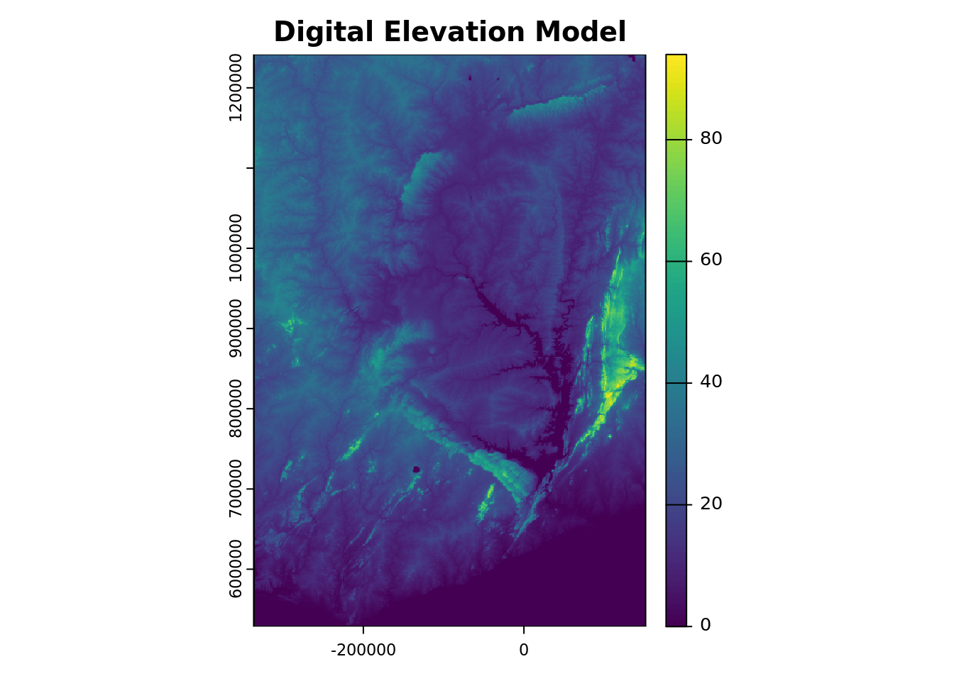
3.3.2 Masking and exploring the covariate stack
The covariate layers were extracted from global layers using a rectangular bounding defined by the extent of the country. For mapping, we aim to restrict the predictions to the country boundary by excluding pixels that fall outside the border. In addition, we want to eliminate pixels representing non-soil areas such as built-up areas and water bodies. In other words, we seek to mask out the areas that are not of interest for mapping. To achieve this, we use a mask layer which is a raster file that delineates the country’s boundary.
# read mask
m <- rast(maskFile)
Masking can be done with the mask() function of the terra package. Similar to rast(), it is essential that the input rasters share the same coordinate system, spatial resolution and extent. Before masking, it’s important to verify that these three attributes are aligned across the layers.
# check that mask and stack have the same:
# coordinate system
crs(r1, describe = TRUE)$name == crs(m, describe = TRUE)$name
[1] TRUE# spatial resolution
res(r1) == res(m)[1] TRUE TRUE# extent
ext(r1) == ext(m)[1] TRUESince all match, we can proceed with mask() function. Keep in mind that masking may take some time to complete, depending on the size of the data and technical specifications of your computer.
# perform masking
r2 <- mask(r1, m)

# inspect the masked stack object
r2
# plot one covariate layer
plot(r2[[elevation_covar_name]],
main = "Digital Elevation Model")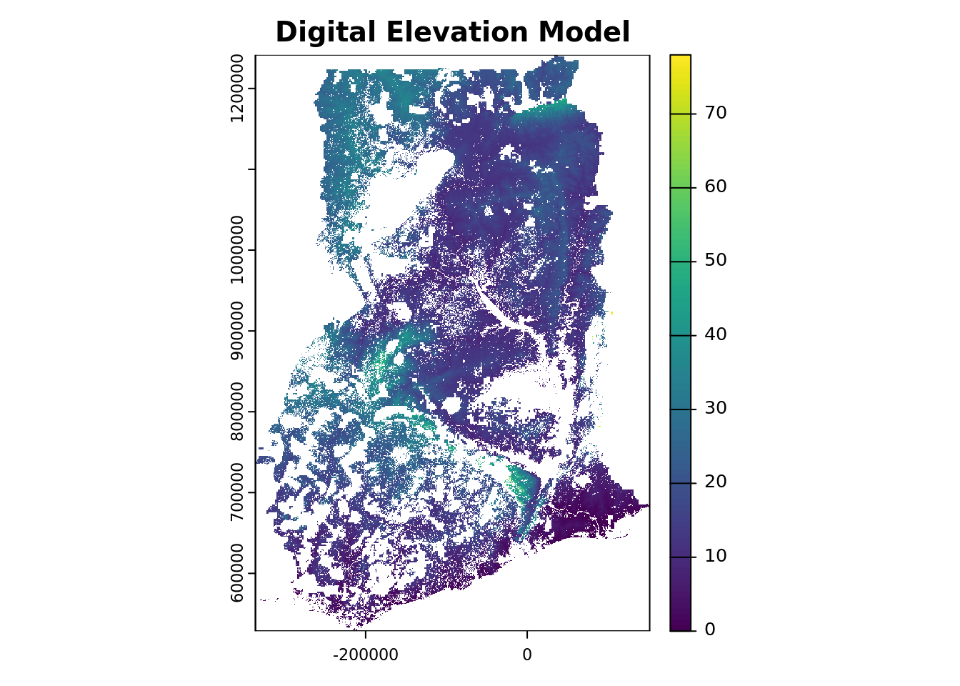
You can now observe that the elevation (and other covariate layers) have been successfully masked, removing both the pixels outside Ghana and the non-soil areas within the country boundary.
Next, proceed by verifying the projection of the raster stack using the crs() function from the terra package.
# check projection
crs(r2, proj = TRUE, describe = TRUE)
name authority code area extent
1 World_Goode_Homolosine_Land <NA> <NA> <NA> NA, NA, NA, NA
proj
1 +proj=igh +lon_0=0 +x_0=0 +y_0=0 +datum=WGS84 +units=m +no_defsThe stack is projected in the Interrupted Goode Homolosine [ESRI:54052] projection with units in meters (m).
3.3.3 Covariate selection through near-zero variance analysis
The next step in the covariate processing workflow is to remove covariates that exhibit little to no variation in their values. Such layers are not informative for modelling, as these do not contribute to explaining any variability in the sample data. Moreover, retaining these layers unnecessarily increases memory usage and slows down computation.
Given the size of the covariate stack, visually inspecting each layer in a GIS environment is impractical. To automate this process, we can use the nearZeroVar() function from the caret package, which identifies variables with zero or near-zero variance. Since this function requires a data.frame as input, the first step is to convert the SpatRaster object to a data.frame format.
# convert SpatRaster to data.frame
r2_df <- as.data.frame(r2, xy = TRUE, na.rm = TRUE)

# run nzv function
nzv <- nearZeroVar(r2_df, saveMetrics = TRUE)
# inspect the output
head(nzv)
# zero variance covariates
summary(nzv$zeroVar)
# near-zero variance covariates
summary(nzv$nzv)The analysis reveals that there are 16 covariate layers with near-zero variance and 12 with zero variance.
These covariates offer little to no value for modeling, so we will remove them from the stack.
The results of the near-zero variance (NZV) assessment is stored in the fourth column of the nzv object, where each entry is either TRUE (indicating the covariate has (near-)zero variance) or FALSE (indicating sufficient variance).
To retain only the informative covariates, we need to invert the results in this column—converting TRUE to FALSE and vice versa. This inverted logical vector is then used to select the appropriate columns from the r2_df data frame, where each column corresponds to a covariate.
To perform this operation, we begin by selecting the fourth column of the nzv object, which contains the logical indicators for zero or near-zero variance. By placing a ! in front of this selection, we invert the logical values. Next, we embed this selection inside a column selection that we apply to the r2_df object.
# drop nzv layers
r2_df <- r2_df[, !nzv[, 4]]
Notice that r2_df now contains 22 covariate columns, in addition ot the “x” and “y” coordinate columns. This means that 12 covariates were identified as having zero or near-zero variance and have been removed from the dataset.
3.3.4 Removing incomplete data pixels
In this section, we will run several checks on the covariate stack to identify any unrealistic or suspicious values. Specifically, we will look for extremely large or small values compared to the quartiles and median. Such values might distort predictions.
# summary statistics
summary(r2_df)
At first glance, the summary statistics do not suggest any suspicious or erroneous values, and there do not appear to be covariates with a high proportion of missing data. It is essential for DSM that every pixel has a value for each covariate. If any covariate contains missing data for certain pixels, predictions cannot be made for those pixels.
With the complete.cases() function, we can identify if there are any missing values in each row of a data.frame like r2_df (note that in our case each row represents a pixel in the map). However, this function should only be applied if the number of missing values is small, otherwise it is better to exclude the entire covariate. Before proceeding with complete.cases(), we first need to determine which columns in r2_df store the covariate values so that we can apply the function to these specifically.
# check names
colnames(r2_df)
In this case, the r2_df object contains only the x and y coordinate columns in addition to the covariates. The complete.cases() function checks for the absence (TRUE) or presence (FALSE) of missing values across the rows of the selected columns. To extract the rows (i.e. pixels) that meet the condition (i.e., those without missing values in the covariates), we can use the subset() function. This will allow us to retain only the rows where all covariate values are present.
# list the columns that store covariate values, i.e. exclude coordinates
covar_cols <- which(!(colnames(r2_df) %in% c("x", "y")))
# check how many incomplete cases there are
nrow(subset(r2_df, !complete.cases(r2_df[covar_cols])))
In this case, we have 0 incomplete cases, i.e. pixels with missing values for one or more selected covariates. The following code lines can be used to remove rows (pixels) with incomplete covariate data.
# subset complete cases
r2_df <- subset(r2_df, complete.cases(r2_df[covar_cols]))
# check number of rows
nrow(r2_df)
Note that if there are no missing values, the number of rows (pixels) will not change.
Now that we are done with covariate processing, the cleaned covariate stackcan be saved to the hard disk as a RDS file.
# save covariate stack
saveRDS(r2_df, file = covarStackFile)
3.4 Regression matrix
This section outlines how to generate a regression matrix in R. The regression matrix is the key input for any digital soil mapping model, as it combines soil observations from sampling sites with values of environmental covariates that act as predictors.
This section is organized as follows:
Section 3.4.2: Loading the input data in R and converting the data into spatial objects.
Section 3.4.3: Performing a spatial overlay of points and covariates to extract the corresponding covariate values at the sampling sites.
Section 3.4.4: Generating the regression matrix.
Section 3.4.5: Removing data points with one or more missing covariate values.
The point data were processed in Section 3.2 and the covariate layers in Section 3.3. This section builds upon the outputs from these previous steps as the input for generating the regression matrix.
3.4.1 Environment preparation
We need the following libraries in this section.
library(sf)
library(terra)
The location of the output files (i.e. that contains the ‘data_preparation’ folder) was defined in Chunk 2.
To begin, we define the objects that store the file paths to the input data files—specifically, the processed covariate stack and the processed soil point data. We use the file.path() function to construct the full file paths by combining the data folder location and the respective file names.
covariateStackFile <-  file.path(outputDir, "covariateStack.rds")
pointDataFile <- file.path(outputDir, "pointData.rds")
Note that although these two data objects are used as input here, these are actually considered outputs of the DSM workflow—having been created during the earlier data preparation steps. We therefore find these input files in the output directory.
Similarly, we will define the name and location of the output files that will be created with this script. In this case, the only output is a file in rds format, which will store the regression matrix.
# location and name of the file that will store the map object
regrMatrixFile = file.path(outputDir,"regressionMatrix.rds")
3.4.2 Reading the input data and creating spatial objects
A digital soil mapping model aims to find predictive relationships between soil observation and environmental covariates, which represent or proxy the soil forming factors, using empirical correlation. To calibrate a DSM model, we need to obtain the covariate values for each sampling site. This is done through a spatial overlay, which results in an object known as the regression matrix.
We start by reading the R objects that store the point data and covariate stack.
# read point data and the covariates stack
d <- readRDS(pointDataFile)
r <- readRDS(covariateStackFile)
To extract covariate values for each data point, we can use the extract() function from the terra package. This function requires a SpatRaster object (which contains the covariate stack) and vectors of coordinates representing the locations where the raster values need to be extracted
Since we prepared the point data with the sf package, the points already have “geometry attached”, but the covariates are still in the non-spatial data.frame format.
class(d)[1] "sf" "data.frame"class(r)[1] "data.frame"To be able to use the extract() function, the points must be converted to SpatVect format and the covariate stack to SpatRaster format.
Let’s start with the first.
d <- vect(d)And continue with converting the covariate stack from data.frame format to SpatRaster format. We use the rast() function for this. The function, however, cannot directly handle a data.frame and needs a matrix as input. A data.frame can be converted into a matrix using the as.matrix() function. The rast() function requires the type argument to be set to xyx to specify that the first two columns in the matrix correspond to the the x and y coordinates (verify this!!), while the remaining columns correspond to the raster layers data. Additionally, the coordinate reference system (CRS) needs to be defined using the crs argument.
We specified the coordinate system for both the points and covariates in Chunk 3. The covariates are projected in the Interrupted Goode Homolosine[ESRI:54052] projection, with units in meters (m). The soil data, on the other hand, is in WGS 84 [EPSG:4326], with units in degrees (°).
# concatenate the covariates crs
crs_covars <- paste0(crs_authority_covar, ":", epsg_number_covar)
# rasterize the data.frame
# note that the rast function requires a matrix as input
r <- rast(as.matrix(r), type = "xyz", crs = crs_covars)
# inspect raster object
rTo match the projections, we can reproject the data using the project() function from the terra package. You can choose whether to reproject the points or the covariates, as this will determine the coordinate reference system for the final outputs. For the sake of convenience in this manual, we will retain the projection of the covariates, as reprojecting the points tends to require less computational power.
Note: If you choose to reproject the covariates, you will find that the project() function for SpatRaster objects inclues an argument called method. You may want to create two separate stacks of reprojected data: one for numeric covariates using a bilinear interpolation, and another for categorical covariates using a nearest neighbor (near) interpolation. For further details, refer to the documentation by running ?terra::project in the console.
# reproject the points
d <- project(x = d, y = r)
The first argument of the project() function specifies the object to be reprojected, while the second argument defines the target coordinate system. The coordinate system can be provided in various formats, or alternatively, you can provide an object from which the function will extract the crs. That’s why, in the previous chunk, r appears in the second argument. By doing so, we ensure that both objects will share the same crs.
3.4.3 Extracting covariate values
Next, we proceed to extract the values of the SpatRaster covariates at the coordinates of the SpatVector points using the extract() function from the terra package.
# spatial overlay
d_cov <- extract(x = r, y = d)
# inspect
class(d_cov)
head(d_cov)
# inspect summary statistics
summary(d_cov)3.4.4 Generating the regression matrix
The results of the spatial overlay give a data.frame (not spatial) containing only the covariate data. To create the regression matrix, we need to combine these extracted values with the measured soil property values of the selected variable, SOC, and the coordinates. The coordinates are stored in object d, with column names orgc and geometry. We select orgc from d and convert the SpatVector to a data.frame using the as.data.frame() function. By specifying the argument geom="XY" we include the coordinates, and store this new object as d_sel. Finally, we append the covariate data in d_cov to d_sel using the cbind() function.
# select variable and coordinates from the points
d_sel <- as.data.frame(d[variable], geom="XY")
# append covariate data to soil data
rgmx <- cbind(d_sel, d_cov)
3.4.5 Removing missing values
The summary statistics indicated that some data points are missing covariate values. This could because the points fall outside the mask, possibly due to the coarse resolution of the covariates (1000m).
Since these data points cannot be used for modelling, we should exclude these from our regression matrix. To do this, we can use the complete.cases() function to find out which data points that have one or more missing covariate values. This function needs to be applied only to the columns containing the covariates, so before using it, we first need to identify which columns in the regression matrix store the covariates.
The d_cov object that we appended to create the regression matrix, contains the covariates names. Only the first column, ID is not a covariate. We will remove this column and save the remaining column names in a vector.
# check which columns store covariates
names(d_cov)

# create covariates names vector
covars_names <- names(d_cov)[-1]
Now we can apply the complete.cases() function to the covariate columns. Let’s first check how many data points are missing covariate data.
# check completeness
summary(complete.cases(rgmx[covars_names]))
The outcome shows that 30 data points are missing covariate data. Now, let’s subset the data to include only the points with complete covariate data.
# select only data points with complete covariate information
rgmx <- subset(rgmx, complete.cases(rgmx[covars_names]))
You are done! Now, save the regression matrix as an R output file.
# save regression matrix
saveRDS(rgmx, file = regrMatrixFile)
# end-of-script