4 Digital Soil Mapping main steps

This chapter demonstrates how to fit a random forest model for soil data and use this model to spatially predict a soil property of interest across a mapping area using the statistical software R. The processing steps are illustrated with a sample dataset. The chapter consists of five sections:

Section 4.2 Model fitting: Fitting a random forest model using the ranger package.

Section 4.3 Recursive feature elimination: Removing redundant covariates from the covariate stack.

Section 4.4 Accuracy assessment: Assessing accuracy statistics of the fitted random forest model.

Section 4.5 Spatial prediction: Applying the model to create a gridded soil map for an area of interest.

Section 4.6 Uncertainty assessment: Calculating the 90% prediction interval with the quantile random forest method.

Note: the five sections form a machine learning ‘workflow’ that should be executed in sequence. Output objects generated in one part typically serve as inputs for the next.

After completing this chapter you will be able to:

Construct a model formula and fit a random forest model with the ranger() function.
Calculate and visualize variable importance statistics.
Perform model selection with the recursive feature elimination method.
Access and interpret random forest accuracy statistics.
Generate predictions of the soil property of interest using the covariate stack as input.
Create a gridded GIS layer in GeoTiff format from the predicted soil values.
Apply quantile random forest to generate uncertainty measures, in particular the 90% prediction interval.

4.1 Set up

The required R packages for this chapter are:

ranger: A fast implementation of Random Forests.
ggplot2: A system for creating elegant data visualizations using the Grammar of Graphics.
dplyr: A Grammar of data manipulation.
caret: Classification and regression training.
terra: Spatial Data Analysis.

At the beginning of each section, the packages to be loaded are specified. If any package is not installed, you can use the install.packages() function to download and install it.

# To check if a package is installed
system.file(package = 'terra')

# it prints the directory where the package is installed
# otherwise, an empty directory is printed as ''

# To install a package uncomment the following line
#install.packages('terra')

The input data for this chapter was processed in the ‘Data Preparation’ chapter of this manual. Specifically, the point data in Section 3.2, the covariate layers in Section 3.3, and and the regression matrix in Section 3.4.

It is considered good practice to avoid hard-coding file paths, file names and variable names in your code. Instead, store these R objects, which can then be reused throughout the code. This makes your code more versatile and easier to adapt. For example, when modeling a different soil property, you only need to change the property name once at the beginning of the code, rather than updating it multiple times throughout the script. This not only saves time but also reduces the risk of errors.

Set the working directory on your local machine. Note that this directory must contain the outputs from Chapter 3.

Chunk 1: Local paths

workingDir <- file.path("C:/tutorials")
folderPath <- file.path(workingDir, "DSM_tutorial")
outputDir <- file.path(folderPath, "output")

Next, we define some variables to make the code more reusable. We create an object to store the name of the soil variable of interest (voi) that we wish to model.

Chunk 2: Variables to explore

# Variable to explore from the points table
# Must be the same as the column name
voi <- "orgc"

# Country name
country <- "Ghana"

# Arguments to be used in text and plots
main <- "SOC"
units <- "%"
xlab <- paste0(main, " (", units, ")") #"SOC (%)"
target_variable <- "Soil Organic Carbon content"

As mentioned in Chunk 2, the target variable for mapping in this manual is Soil Organic Carbon content ( SOC (%) ) in Ghana. This variable is stored in column called orgc in our dataset (the regression matrix).

We need to set a random seed to ensure our results are reproducible. Keep in mind that the random forest algorithm uses bootstrapping to sample data and randomly selects covariates for splitting. As a result, each time you fit a random forest model on your data, the outcomes may vary slightly.

The random seed can be set with the set.seed() function. The number you choose can be any integer. By doing this, we guarantee that the results will be the same each time the code is run.

Chunk 3: Set seed

set.seed(20180523)

For Section 4.5 and Section 4.6 we will need two additional folders within the output folder. Note that these directories must already exist in the working directory, as the code below does not create them.

Chunk 4: Output figures and maps folders

outputDir_figs = file.path(outputDir,"figures/")
outputDir_maps = file.path(outputDir,"maps/")

For Section 4.5 and Section 4.6, we also define an object to store the coordinate reference system of the covariates.

Chunk 5: Covariates coordinate system

# Coordinate system of covariates
coord_system_covar <- "Interrupted Goode Homolosine"
epsg_number_covar <- 54052
crs_authority_covar <- "ESRI"

The coordinate system of the covariates is the Interrupted Goode Homolosine. The EPSG code for this projection is Interrupted Goode Homolosine. The terra package supports EPSG codes when using the following notation: <authority>:<code>, which in this case is “ESRI:54052”. We also create an object to store this notation for reuse in the code.

crs_epsg_covar <- paste0(crs_authority_covar, ":", epsg_number_covar)

The following global option will prevent very large numbers—such as coordinates in projected systems—from being displayed in scientific notation.

# to avoid scientific notation
options(scipen=999)

4.2 Model fitting

This section shows how to fit a random forest model in R and includes the following steps:

Section 4.2.1: Loading the input data in R.
Section 4.2.2: Creating a model formula and fitting a random forest model with the ranger() function.
Section 4.2.3: Inspecting model output and variable importance analysis.

The following libraries are required for this section:

# load libraries
library(ranger)
library(ggplot2)

We now define an objects that stores the file path to the input data: in this case the regression matrix created in Section 3.4. We use the file.path() function to construct the full file path.

# define file path of the file storing the regression matrix
regrMatrixFile = file.path(outputDir, "regressionMatrix.rds")

Similarly, we define the name and location of the output file generated in this section. In this case, a single R output file in rds file format will be created. It will contain the fitted random forest model and will be saved in the output folder in the working directory.

# file name of the fitted random forest model
modelFile = file.path(outputDir, paste0("rfModel_", voi, ".rds"))

Note that the name of the variable of interest (stored in the object voi) is included in the name of the rds output file that stores the fitted random forest model. This ensures that a separate file is saved for each soil property that is modeled, preventing output files from being overwritten. The paste() function is used to concatenate the different components of the output file together.

4.2.1 Reading the regression matrix

In this manual, we will fit a random forest model for SOC. We begin by reading the input data, which are the soil sample data along with their associated covariate values, i.e. the regression matrix. This matrix was generated in Section 3.4.

# read regression matrix
rgmx <- readRDS(regrMatrixFile)

4.2.2 Fitting a random forest model

We use the ranger() function of the ranger package to fit a random forest model. The ranger package provides a faster implementation of the random forest algorithm compared to the randomForest package. Furthermore, it offers some additional functionality, such as quantile random forest for quantifying prediction uncertainty.

You can view the help file of the ranger() function by typing ?ranger in the console. The Usage section in the documentation lists the function arguments.

The only two mandatory arguments for the ranger() function are:

formula: an object of class formula that defines the model to be fitted.
data: a data.frame containing the training data (i.e. the regression matrix)

The formula is in form of soil_variable ~ covariate1 + covariate2 + ... + covariate_n.

Since we have 22 covariates, manually typing each covariate name to define a model formula would be cumbersome. Instead, we can construct the model formula efficiently using the paste0() function, which allows you to concatenate individual elements into a single string.

Let us first look at the elements needed to form a formula string. The first element is the name of the soil variable we wish to model. The second element is the tilde (~), which you could read like variable explained by. The third element consists of a series of covariate names separated by a ‘+’.

We begin by extracting the covariate names from the regression matrix. The first covariate is stored in column 5, and the total number of columns in the matrix is 26. We select the relevant columns from the regression matrix object rgmx, and then extract the column names with the names() function.

# store covariate names in a separate object
covar_names <- names(rgmx[ ,5:ncol(rgmx)])

# inspect object
covar_names

We continue with pasting the covariate names together in a single text string with the paste() function. If we pass " + " to argument collapse, then the function will connect the separate elements (i.e. the covariate names) with a ‘+’ sign.

# construct covariate string
covar_string <- paste(covar_names, collapse = " + ")

# inspect object
covar_string

Now we can concatenate the three parts using paste(): the name of the variable of interest (stored in the voi object), the tilde and the covariate string.

formula_string <- paste(voi, " ~ ", covar_string)

# inspect object
formula_string

# check class
class(formula_string)

The final step is to convert the formula string from a plain character object into a formula object.

# convert to formula object
mod_for <- as.formula(formula_string)

# show formula and object class
mod_for
class(mod_for)

Note that while we used a step-by-step approach to construct the model formula, the same result could be achieved in a single line of code using nested functions.

# create model in one line
mod_for <- as.formula(paste(voi, "~", paste(covar_names, collapse = " + ")))

We proceed to fit a random forest model in its most simple format. The model fitting process is controlled by key parameters: ntree and mtry. It is not necessary to specify these parameters. If not provided, R will use the default values.

In ranger, it is also important to define the method to assess variable importance using the importance argument. If not specified, variables importance will not be computed. The impurity measure calculates the Gini index for classification (categorical variables) and the variance of the responses for regression (continuous variables). This is the most commonly used option.

Now, we will continue with fitting a random forest model using the default ntree and mtry values.

# fit the model
rf_model <- ranger(
    formula = mod_for, 
    data = rgmx,
    importance = "impurity"
)

4.2.3 Inspecting model output and variable importance

Let’s check the model output. The output object is quite extensive, so we limit the printing of the output to the second level of nesting by setting the max.level argument.

# inspect rf_model
str(rf_model, max.level = 2)

Inspect the output and try to understand what each of the output arguments means. Check the documentation of the ranger() function and look under the Value section that describes the output arguments.

One important output is stored in the predictions element. This contains the out-of-bag (semi-independent) model predictions at the data points. By comparing these predictions with the observed (measured) values in the regression matrix, you can compute validation statistics that quantify model’s performance.

To view a condensed summary of the model, simply type the object name in the console.

rf_model

Ranger result

Call:
 ranger(formula = mod_for, data = rgmx, importance = "impurity") 

Type:                             Regression 
Number of trees:                  500 
Sample size:                      580 
Number of independent variables:  22 
Mtry:                             4 
Target node size:                 5 
Variable importance mode:         impurity 
Splitrule:                        variance 
OOB prediction error (MSE):       0.105687 
R squared (OOB):                  0.4785321

The randomForest package has a function to create a variable importance plot, but unfortunately, such a function does not exist for ranger. We need to program this ourselves.

We start by extracting the variable importance statistics of the fitted random forest model and store these in a new data.frame. Next, we create a variable importance plot using the ggplot() function of the ggplot2 package.

# create data.frame with variable importance statistics
imp <- data.frame(
  variable = names(rf_model$variable.importance),
  importance = rf_model$variable.importance,
  row.names = NULL
)

# display object content
head(imp)

# plot importance
ggplot(data = imp,
       aes(
         x = reorder(variable, importance),
         y = importance,
         fill = importance
       )) +
  geom_bar(stat = "identity", position = "dodge") +
  coord_flip() +
  ylab("Variable Importance") +
  xlab("") +
  ggtitle(paste("RF model, ", xlab, " - ", country)) +
  guides(fill = "none") +
  scale_fill_gradient(low = "#FBBE5E", high = "#8B2822") +
  theme_minimal()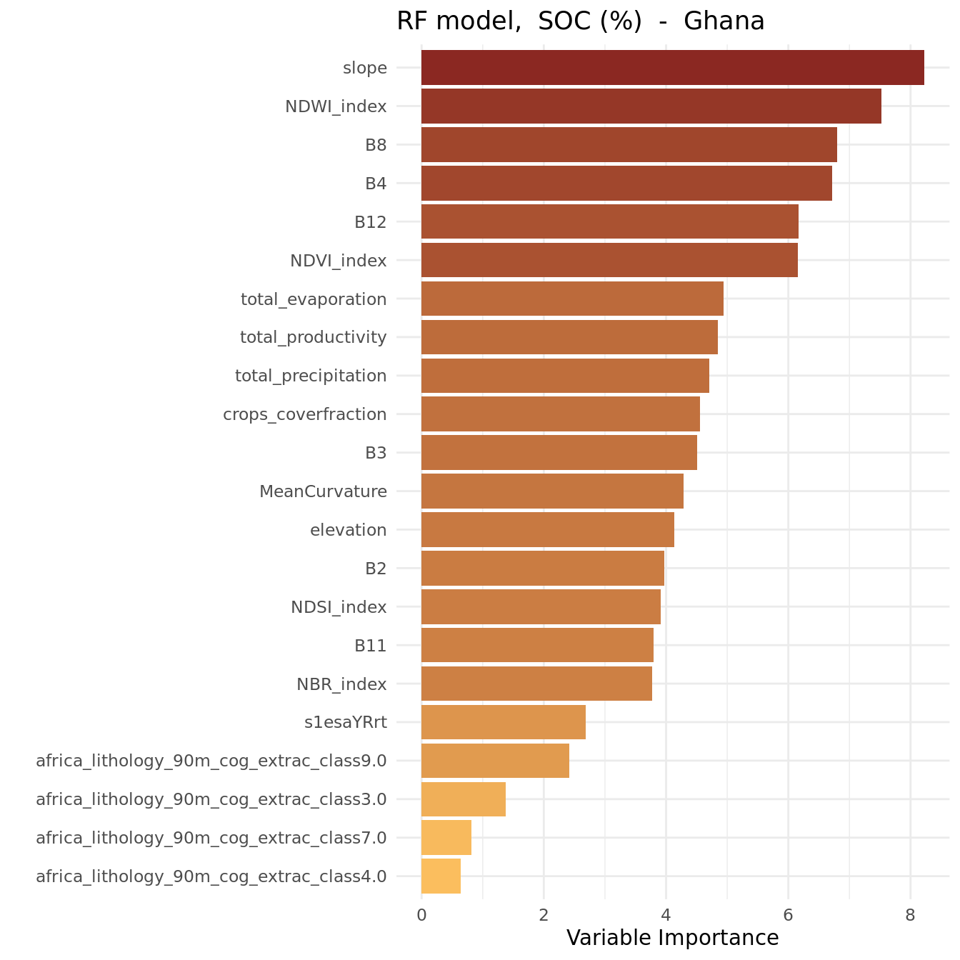

The plot shows that the most important variables (i.e. the strongest predictors) were:

slope
NDWI_index
B8, B4, B12

NDWI stands for Normalized Difference Water Index.

We are done, save the fitted random forest model to the hard disk as an RDS file.

# save fitted model to file
saveRDS(rf_model, modelFile)

# Model fitting
# end-of-script

4.3 Recursive Feature Elimination (RFE)

The number of covariate layers considered in this tutorial is relatively small. However, with the increasing availability of (free) satellite imagery and other sources of biophysical data layers, it is now possible to assemble a covariate stack that includes hundreds of layers. Using such a large stack for spatial prediction with a DSM model can become computationally expensive, especially when predictions are needed at high spatial resolution and for large areas.

Furthermore, some covariate layers in the stack may be (strongly) correlated, particularly those from climatic or vegetation index time series. Several studies caution against using correlated covariates, as these might introduce bias into variable importance measures. Therefore, it is often beneficial to reduce the dimensionality of the covariate stack before performing spatial predictions. One method for covariate selection is a technique called Recursive Feature Elimination (RFE).

RFE is a feature (covariate) selection technique that works by fitting a model and iteratively removing the least important feature(s) until a pre-defined number of features is remains. Features are ranked by the model’s feature importance attributes. By recursively eliminating the least important features, RFE helps reduce redundancy and collinearity.

RFE requires specifying the number of features to retain; however, this number is often not known in advance. To determine the optimal number of features, cross-validation is used to evaluate different feature subsets and identify the one that performs best.

This section shows how to:

Section 4.3.2: Prepare input objects for RFE.
Section 4.3.3: Perform RFE using the rfe() function from the caret package, and assess the outcome using profile plots.
Section 4.3.4: Fit a random forest model using an “optimal” covariate subset.

More details about RFE are available on the website of the caret package

4.3.1 Environment preparation

The following libraries are required for this section:

# load libraries
library(ranger)
library(caret)
library(dplyr)

We already set the working directory in Chunk 1, which is the same directory where the outputs from the previous sections have been saved.

We declared our voi, SOC (%) in this case, in Chunk 2.

To ensure that your output matches ours, we initialized the random number generator by setting a random seed in Chunk 3. Remember, the random forest algorithm (used in RFE) relies on random processes such as bootstrapping sample data and randomly selecting covariates for node splitting. These steps introduce variability into each model run, meaning that each time you fit a random forest model to your data, the results will be (slightly) different.

By using the set.seed() function, we make the model results reproducible. The argument passed to set.seed() can be any number. Once set, it ensures that every time the code is run, it produces the same results.

The caret package contains only pre-defined functions for random forest modelling with the randomForest package (rfFuncs). To be able to use RFE with ranger, we need to load these model functions first. We have saved these functions in script rangerFuncs.R that is provided below. The functions were obtained from the caret github repository.

Unfold the next chunk and run the code.

rangerFuncs.R

# Modified and derived from here https://github.com/topepo/caret/issues/555
library(caret)
rangerFuncs <-  list(summary = defaultSummary,
                     fit = function(x, y, first, last, ...) {
                       loadNamespace("ranger")
                       dat <- if(is.data.frame(x)) 
                         x else as.data.frame(x)
                       dat$.outcome <- y
                       ranger::ranger(.outcome ~ ., data = dat, 
                                      importance = "impurity", 
                                      probability = is.factor(y),
                                      write.forest = TRUE,
                                      ...)
                     },
                     pred = function(object, x)  {
                       if(!is.data.frame(x)) x <- as.data.frame(x)
                       out <- predict(object, x)$predictions
                       if(object$treetype == "Probability estimation") {
                         out <- cbind(pred = colnames(out)[apply(out, 1, which.max)],
                                      out)
                       } 
                       out
                     },
                     rank = function(object, x, y) {
                       if(length(object$variable.importance) == 0)
                         stop("No importance values available")
                       imps <- ranger:::importance(object)
                       vimp <- data.frame(Overall = as.vector(imps),
                                          var = names(imps))
                       rownames(vimp) <- names(imps)
                       
                       vimp <- vimp[order(vimp$Overall, decreasing = TRUE),, drop = FALSE]
                       vimp
                     },
                     selectSize = pickSizeBest,
                     selectVar = pickVars)

We now define objects that store the file paths to the input data files: in this case the regression matrix. Although this file is used as input in this section, the regression matrix is considered an output of the DSM workflow created during the data preparation in Section 3.4. Therefore, the file is located in the output directory of the working environment.

# define file path of the file storing the regression matrix
regrMatrixFile = file.path(outputDir, "regressionMatrix.rds")

Similarly, we define the name and location of the output files (in rds file format) that are generated in this section. One will store the fitted random forest after running RFE, and the other will store the output of the RFE run.

# output file name to store the fitted random forest model with rfe
modelFile_rfe = file.path(outputDir, paste0("rfModel_", voi, "_rfe.rds"))

# output file name to store the fitted rfe profile
rfeProfileFile = file.path(outputDir, paste0("rfeProfile_", voi, ".rds"))

Note that the name of the variable of interest (stored in the object voi) is included in the name of the rds output files. This ensures that separate files are saved for each soil property that is modeled, preventing output files from being overwritten. The paste() function is used to concatenate the different components of the output file together.

4.3.2 Read data and prepare RFE inputs

Start with loading the regression matrix in our R session.

# read regression matrix
rgmx <- readRDS(regrMatrixFile)

The rfe() function requires four input objects:

A matrix or data.frame object with the covariates.
A vector object with the training data (i.e. the soil property to be modeled).
A vector object specifying the sizes of covariate subsets to evaluate.
A list of control options for configuring the RFE process.

As a next step, we are going to create these these objects. We start with the covariate object. We need to extract the covariates from the regression matrix, so we need to identify which columns store the covariate data. Let’s take a look at the column names.

# display column names
names(rgmx)

We can observe that the first covariate is stored in column 5 (feel free to verify this!), and the regression matrix contains a total of 26 columns. To extract the covariate columns, we can use the select() function from the dplyr package, specifying the relevant column numbers.

# store covariates in separate object
covars <- select(rgmx, 5:ncol(rgmx))

Continue to select the column storing the values of the variable of interest. Note that we do not use the select() function here because it returns a data.frame, whereas we need a vector object.

# store soil data values in a separate object
training <- rgmx[,voi]

Next, we create an object as input for the the sizes argument in the rfe() function. This argument requires a vector with integer values representing the specific subset sizes to be tested. The sizes used here are only a suggestion and a compromise between accuracy and speed. If time and computational power are not a constraint, a larger number of subset sizes should be tested.

# define subset sizes to test
sizes <- unique(c(seq(6, 15, 3), seq(15, length(covars), 5), length(covars)))
sizes

[1]  6  9 12 15 20 22

The rfe() function uses the rfeControl argument to configure RFE options, which are specified with the rfeControl() function. This function has the following arguments:

functions: A set of functions used for model fitting, prediction and variable importance for specific models. The package provides a number of pre-defined function sets for several models, including linear regression and random forest.
method: The resampling method used to assess performance of each covariate subset.
number: Either the number of folds or number of resampling iterations for the chosen method.
saveDetails: A logical argument indicating whether to save the predictions and variable importance during the selection process.

You can access the help file of this function by running ?rfeControl if you like more details.

# define rfe parameters with the rfeControl function
ctrl <- rfeControl(
    functions = rangerFuncs,
    method = "repeatedcv",
    number = 2,
    returnResamp = "all",
    saveDetails = TRUE,
    verbose = FALSE
)

To ensure efficiency, we use a 2-fold cross-validation approach. For more robust modelling and evaluation of model performance across different feature subset sizes, you may consider increasing the fold number (e.g. to 5).

4.3.3 Run RFE and inspect results

Now we are ready to run RFE and inspect the results. Please note this process might take some time, so we may need to be patient.

# run RFE
rf_profile <- rfe(
  x = covars,
  y = training,
  sizes = sizes,
  rfeControl = ctrl
)

# view object class
class(rf_profile)

# inspect output
rf_profile

# view selected covariates
predictors(rf_profile)

The output provides accuracy statistics (root mean squared error, R-squared, mean absolute error) for each of the tested covariate subset sizes. The subset with the smallest RMSE value is selected as the “best” subset size.

The predictors() function returns the covariates that are included in this best subset. For more detailed information, you can use str() function. Summary information about the model fitted with the selected subset size can be found under the fit element (rf_profile$fit).

Additionally, there are also several plotting methods to visualize the results. The plot(rf_profile) function generates a performance profile across different subset sizes for different metrics, as shown in the figures below.

# RFE plots
plot(rf_profile, metric = "Rsquared", type = c("g", "o"))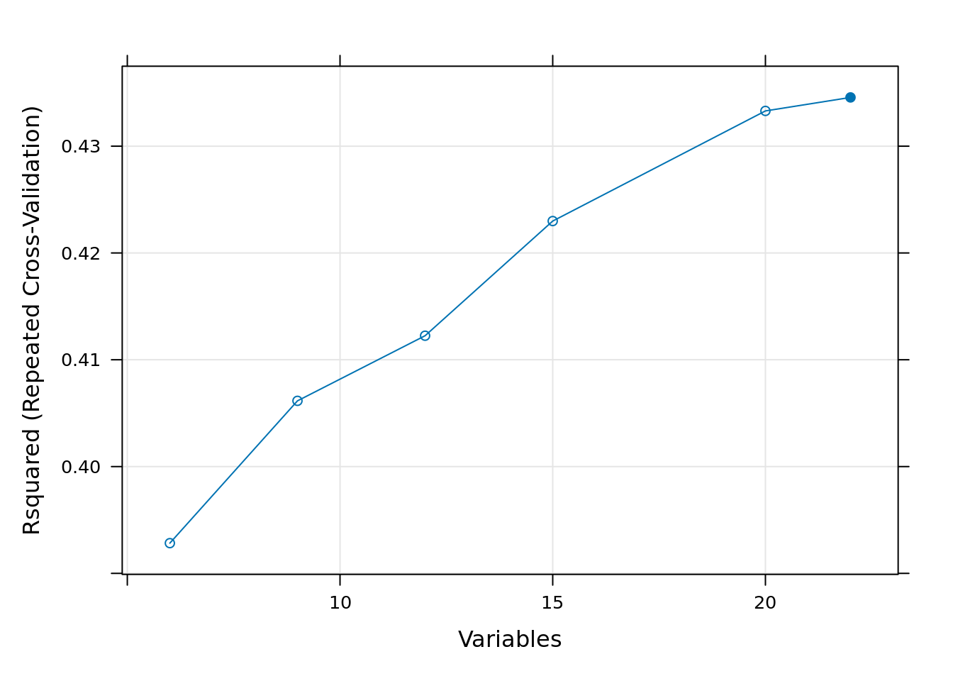

plot(rf_profile, metric = "RMSE", type = c("g", "o"))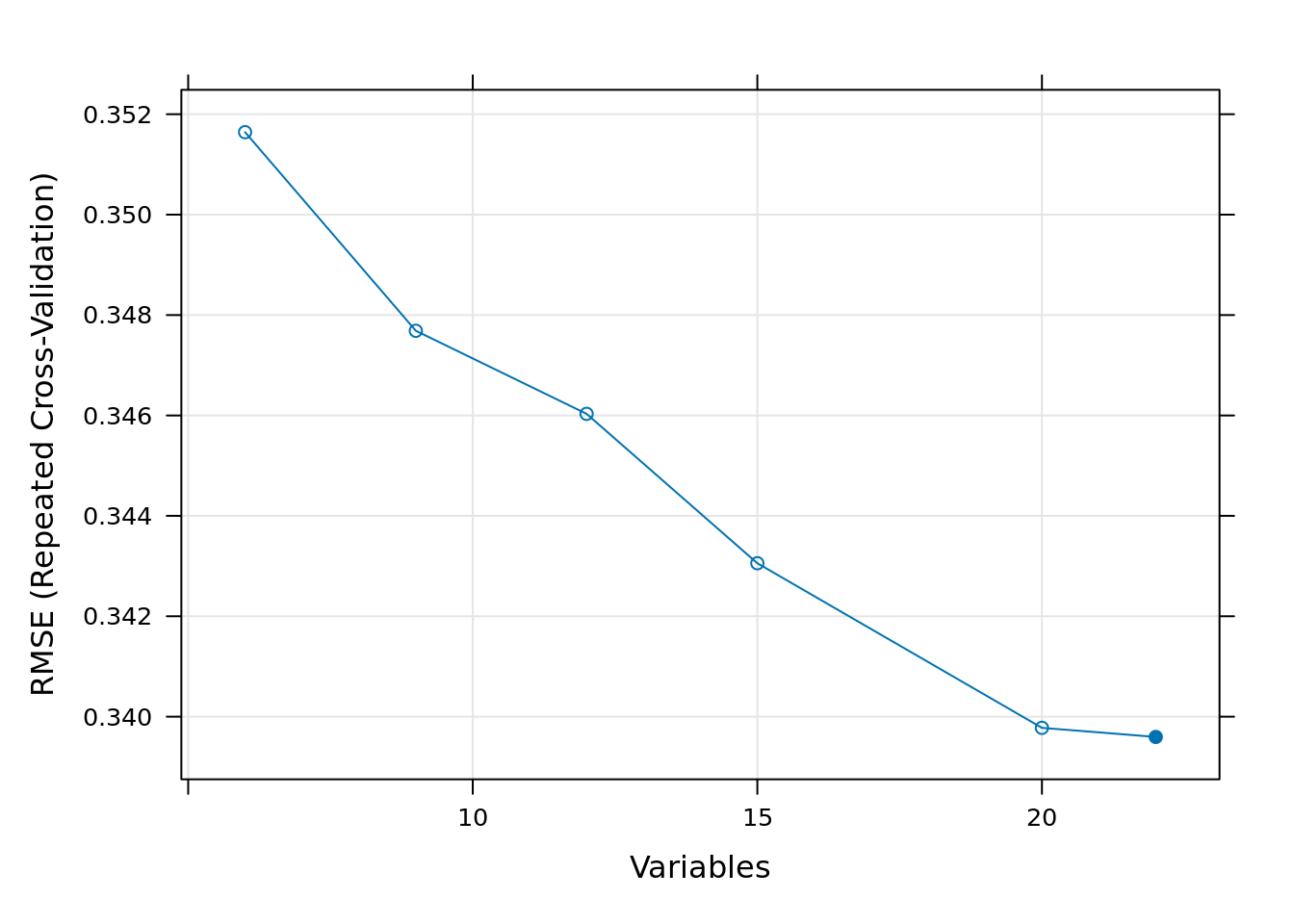

We note that differences in model performance between different subset sizes are generally very small, except for really small subset sizes. The main reason using RFE for variable selection is not necessarily to improve model accuracy, but to increase computational efficiency—making random forest modeling and spatial prediction faster and less memory-intensive.

For this reason, we have decided to select the first 20 variables for fitting the model, because when analyzing the graphs it can be seen that around the 20 variables onward, the Rsquared and the RMSE change relatively little.

# store selected covariates in a new object
covars_rfe <- predictors(rf_profile)[1:20]

4.3.4 Fit RF model based on RFE outcome

Now that we have determined the “optimal” covariate subset, we can refit a random forest model using only this subset as input. As in the previous section (Section 4.2), we first construct a model formula that we can pass on the the ranger() function. To do this, we use the predictors() function to extract the names of the covariates of the optimal subset and store these in a new object. We then use this object to create the model formula.This can all be done in one step using nested functions. For a more detailed explanation on how to construct a model formula, refer to See Section 4.2.2.

# define model formula
mod_for_rfe <- as.formula(paste0(voi, "~", paste(covars_rfe, collapse = " + ")))

# inspect object
mod_for_rfe

# refit the random forest model
rf_rfe <- ranger(formula = mod_for_rfe,
                 data = rgmx,
                 importance = "impurity")

We conclude this section by making a variable importance plot in the same way as done before.

# create data.frame with variable importance statistics
imp_rfe <- data.frame(
    variable = names(rf_rfe$variable.importance),
    importance = rf_rfe$variable.importance,
    row.names = NULL
)

# plot importance
ggplot(data = imp_rfe,
       aes(
         x = reorder(variable, importance),
         y = importance,
         fill = importance
       )) +
  geom_bar(stat = "identity", position = "dodge") +
  coord_flip() +
  ylab("Variable Importance") +
  xlab("") +
  ggtitle(paste("RF model - RFE, ", xlab, "- ", country)) +
  guides(fill = "none") +
  scale_fill_gradient(low = "#FBBE5E", high = "#8B2822") +
  theme_minimal()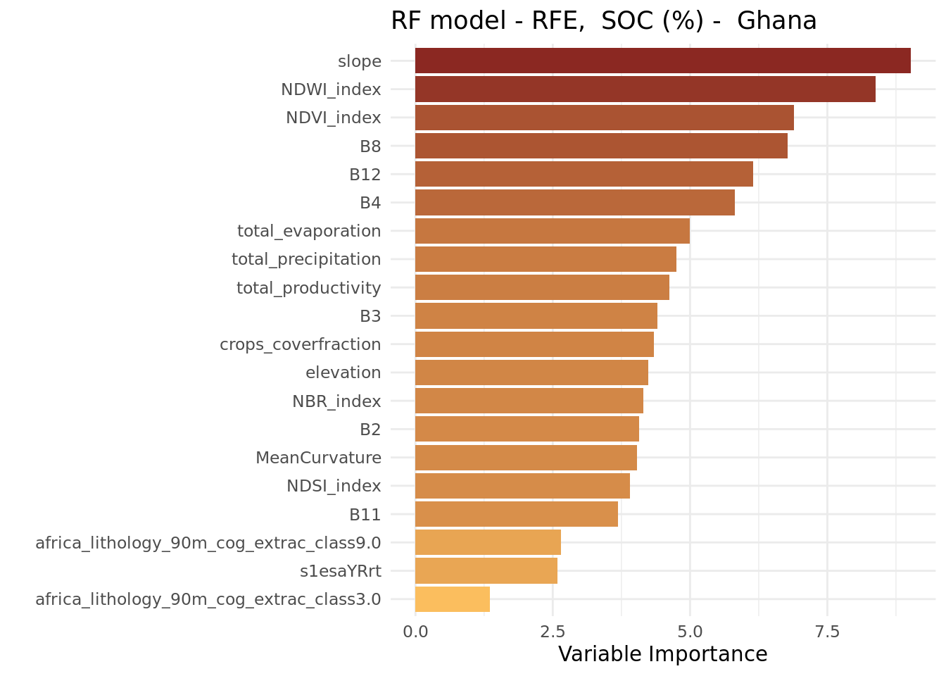

We observe that the variable importance order does not differ much from that of the ranger model that included all covariates.

With the analysis complete, we now save the results of the RFE process, as well as the newly fitted random forest model, to disk.

# save rfe profile to file
saveRDS(rf_profile, rfeProfileFile)

# save fitted model to file
saveRDS(rf_rfe, modelFile_rfe)

# RFE
# end-of-script

4.4 Accuracy assessment

Once a prediction model has been trained, it is important to assess how well it fits the data. The random forest model output includes some easily accessible goodness-of-fit statistics. This section will show how to access these statistics and compares the performance models fitted with and without RFE.

4.4.1 Environment preparation

The following libraries are required for this section:

# load libraries
library(ranger)

We already set the working directory in Chunk 1. It is the same one in which you have saved the outputs from the previous sections.

Our variable of interest (VOI), SOC (%), was defined in Chunk 2.

We now define objects to store the file paths for the input data: in this case the regression matrix and the fitted random forest models (with and without RFE). Although these objects are used as input in this section, these are all considered outputs of the DSM workflow generated in earlier parts of this manual. As such, these are located in the output directory. We use the file.path() function to create a full file path by combining the output folder path with the respective file names.

# define file path of the file storing the fitted RF model
modelFile = file.path(outputDir, paste0("rfModel_", voi, ".rds"))

# define file path of the file storing the fitted RF model with RFE
modelFile_rfe = file.path(outputDir, paste0("rfModel_", voi, "_rfe.rds"))

# define file path of the file storing the regression matrix
regrMatrixFile = file.path(outputDir, "regressionMatrix.rds")

# output file name to store the fitted random forest model with rfe
accStatsFile = file.path(outputDir, paste0("accStats", voi, ".csv"))

4.4.2 Read data

Start with reading the three data objects in your R session.

# read RF model
rf_model <- readRDS(modelFile)

# read RF model fitted with RFE
rf_rfe <- readRDS(modelFile_rfe)

# read regression matrix
rgmx <- readRDS(regrMatrixFile)

4.4.3 Accessing accuracy statistics

A good starting point for accuracy assessment is to plot the predicted values at the training points against the observed values. The predicted values are out-of-bag (OOB) predictions, which are stored in the element predictions in the ranger model object. The observed (measured) values, however, are not included in the model object and must be retrieved separately from the regression matrix.

# inspect the model object
str(rf_model, max.level=2) # note the element 'predictions'

# create a scatter plot
plot(x = rf_model$predictions, 
     y = rgmx[, voi], # selects the observed values from the regression matrix.
     xlab = paste0("Predicted ", xlab),
     ylab = paste0("Observed ", xlab)
)
abline(0, 1) # adds the 1:1 line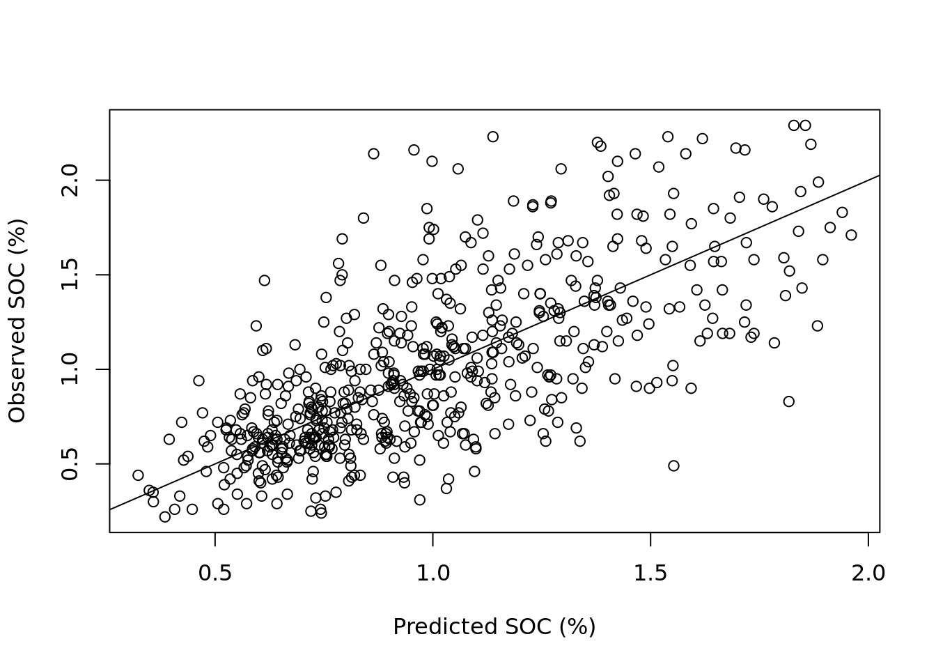

The plot shows correlation between observed and predicted values, but also reveals substantial scatter around the 1:1 line. Notably, predictions for higher values of SOC tend to deviate more from the 1:1 line, suggesting reduced model performance for larger concentrations. The model fit could potentially be applying a log-transformation to the SOC values.

The ranger output includes the OOB mean squared error (MSE), which is a measure of accuracy, and the R² , which indicates which indicates the proportion of the variance in the observed data that is explained by the model (i.e., it is a variance reduction statistic). The MSE is stored under element prediction.error, and the R² under element r.squared. The root mean squared error (RMSE), which reflects the average prediction error in the original units, can be calculated as the square root of the MSE. Next, we will access these statistics, rounding them to two decimal places.

# MSE
round(rf_model$prediction.error, digits = 2)

[1] 0.11

# r-squared
round(rf_model$r.squared, digits = 2)

[1] 0.47

# RMSE
round(sqrt(rf_model$prediction.error), digits = 2)

[1] 0.33

4.4.4 Accessing accuracy statistics after RFE

The previous chunk can be run again but now for the model using only the covariates selected with the RFE.

# MSE
round(rf_rfe$prediction.error, digits = 2)

[1] 0.11

# r-squared
round(rf_rfe$r.squared, digits = 2)

[1] 0.48

# RMSE
round(sqrt(rf_rfe$prediction.error), digits = 2)

[1] 0.33

The statistics show that the difference between the models fitted with and without RFE are negligible. Hence, the primary purpose of RFE is to increase computational efficiency.

The two outcomes can be compared in a plot.

# Get covariates names from the model
covars_rfe <- names(rf_rfe$variable.importance)

dot_colors <- c("black", "blue")

# plot measured values vs random forest predictions
plot(x = rf_model$predictions, 
     y = rgmx[, voi],
     col = dot_colors[1],
     xlab = paste0("Predicted ", xlab),
     ylab = paste0("Observed ", xlab)
)
# add predictions using RFE
points(x = rf_rfe$predictions, 
       y = rgmx[, voi],
       col = dot_colors[2]
)

# Add legend
legend("topleft",
       legend = c("no RFE", "with RFE"),
       col = dot_colors,
       pch = 1)

# Add 1:1 line
abline(0, 1)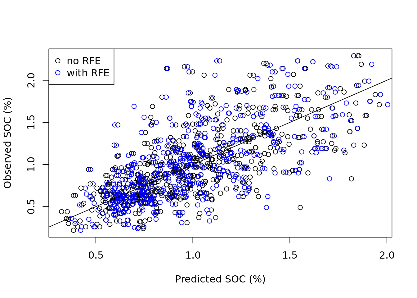

The plot shows that while there are differences between the predictions of the two models, these differences are minor as expected. Both scatter plots have similar shape.

4.4.5 Compiling accuracy statistics

Below we show how to compile the OOB accuracy statistics in a data.frame object, which can then be saved to the hard disk as a table. The resulting data.frame contains two columns: noRFE and withRFE and each contain three accuracy statistics.

acc_stats <- data.frame(
    noRFE = c(
        round(rf_model$prediction.error, digits = 3),
        round(rf_model$r.squared, digits = 3),
        round(sqrt(rf_model$prediction.error), digits = 3)
    ),
    withRFE = c(
        round(rf_rfe$prediction.error, digits = 3),
        round(rf_rfe$r.squared, digits = 3),
        round(sqrt(rf_rfe$prediction.error), digits = 3)
    )
)

# add row.names to data.frame
row.names(acc_stats) <- c("MSE", "R2", "RMSE")

# display results
acc_stats

     noRFE withRFE
MSE  0.106   0.106
R2   0.475   0.478
RMSE 0.326   0.325

Save the statistics table to disk as a csv file.

# write statistics overview to csv table
write.csv(acc_stats, file = accStatsFile)

Note that the OOB validation statistics of the random forest model fitted after running a RFE are slightly different from the validation statistics obtained from the rfe output object rf_profile$fit (see Section 4.3.3). This difference is caused by the fact that we ran the rfe function with a different validation method (2-fold cross-validation).

# Accuracy assessment
# end-of-script

4.5 Spatial prediction

This section shows how to use a digital soil mapping model to create a gridded soil map in R and includes the following steps:

Section 4.5.3: Generating predictions using the random forest model.
Section 4.5.4 and Section 4.5.5: Creating a spatial raster object from the predictions.
Section 4.5.6: Exporting the gridded map as a GeoTiff file.
Section 4.5.7: Saving the prediction as a terra raster object.

The input data for this tutorial were generated in previous sections, specifically in Section 3.3, and Section 4.2. This section uses the outputs of these, stored as R output files (.rds), as input for spatial prediction.

4.5.1 Environment preparation

The following libraries are required for this section:

# load libraries
library(terra)
library(ranger)

We already set the working directory in Chunk 1. It is the same one in which you have saved the outputs from the previous sections.

Our variable of interest (VOI), SOC (%), was defined in Chunk 2.

For this section, we will need to indicate the locations of figures and maps folders as shown in Chunk 4

We now define objects that contain the file paths to the input data files: in this case the covariate stack and the fitted random forest model. Although these objects are used as input in this section, these are all considered outputs of the DSM workflow generated in earlier parts of this manual. As such, these are located in the output directory. We use the file.path() function to create a full file path by combining the output folder path with the respective file names.

covariateStackFile <- file.path(outputDir, "covariateStack.rds")
modelFile_rfe <- file.path(outputDir, paste0("rfModel_", voi, "_rfe.rds"))

In the same way, we define the name and location of the output files that are created in this section. We will create an R output file in rds format that will store the map object, a PNG file of the map and a raster GIS layer in GeoTiff format. These files will be saved in the output directory we’ve been working with. Additionally, we will create two sub-folders within the output directory to organize and store these PNG and GeoTiff files.

mapFile = file.path(outputDir, paste0("rfMap_", voi, ".rds"))
pngFile = file.path(outputDir_figs, paste0(voi, ".png"))
tiffFile = file.path(outputDir_maps, paste0(voi, ".tiff"))

In Chunk 5 we defined the coordinate system of the covariates.

4.5.2 Read the input data

Our goal is to map a soil property of interest across Ghana using a grid with a spatial resolution of 1 km. This implies that a value will be predicted for each pixel in the grid. The prediction location is the center of the pixel.

Two data objects are required for spatial prediction (mapping) of a soil property with a DSM model:

the fitted model
the processed covariate stack.

# read the fitted random forest model
rf_rfe <- readRDS(modelFile_rfe)

# read the covariate stack
cs <- readRDS(covariateStackFile)

If you examine the structure of the cs object closely, you will notice that this object (the covariate stack) is stored as a data.frame, meaning it is in a non-spatial tabular format. Since predictions can be made using a data.frame as input, it is not necessary to convert this object to a spatial format at this stage.

4.5.3 Predict the soil property of interest

We can use the generic predict() function to predict the soil property of interest at the grid nodes across Ghana by applying the random forest model to the covariate stack.

When predicting with a ranger model using the predict() function, two additional arguments must be specified alongside the model object:

data: A data.frame containing the covariate values for the locations where predictions are to be made. Each row represents a grid cell (i.e., a prediction location), and each column corresponds to a covariate used in the model.
type: Specifies the type of prediction. The default is response, which returns predicted values for regression models (continuous variables) or class labels for classification models (categorical variables). Alternatively, quantiles can be used when estimating quantiles of the predictive distribution, which is useful for assessing uncertainty.

In addition to these two arguments, several other options are available for prediction. For example, you can obtain predictions from each individual tree in the forest by setting the argument predict.all = TRUE. For more details, consult the help file for predict.ranger.

Now generate predictions and inspect the results—for example, check whether any predicted values are negative or otherwise unexpected.

# predict
prd <- predict(rf_rfe, data = cs, type = "response")

# inspect output
class(prd)

[1] "ranger.prediction"

str(prd)

List of 5
 $ predictions              : num [1:147012] 0.974 0.82 0.814 0.878 0.901 ...
 $ num.trees                : num 500
 $ num.independent.variables: num 20
 $ num.samples              : int 147012
 $ treetype                 : chr "Regression"
 - attr(*, "class")= chr "ranger.prediction"

summary(prd$predictions)

   Min. 1st Qu.  Median    Mean 3rd Qu.    Max. 
 0.3466  0.8761  1.0020  1.0361  1.1688  2.0914

4.5.4 Compiling the predictions

The predict() function returns an object of class ranger.prediction, with the predicted values stored in the first element. However, since this object is not spatial (it lacks coordinate information) it cannot yet be visualized as a gridded map.

As first step towards creating a spatial R object that can eventually be saved as a GIS file, the predicted values must be combined with their corresponding coordinates and then stored in a new object. This can be done with the data.frame() function. The coordinates can be obtained from the covariate stack cs.

# compile predictions
p <- data.frame(x = cs$x, y = cs$y, pred = prd$predictions)

# change the name of the column containing the predictions to the variable name
names(p)
names(p)[3] <- voi
names(p)

# inspect object
head(p)

4.5.5 Creating a spatial raster object

The predictions are now stored in a data.frame object along with the coordinates. To create a map, we need to convert the data.frame into a spatial raster object, in this case a SpatRaster, which is a class of the terra package.

We can convert a data.frame to a SpatRaster with the rast() function. However, the rast() function cannot handle a data.frame directly as input. Instead it requires a matrix object. We can convert a data.frame to a matrix with the as.matrix() function and then pass it to rast().

In addition, we need to specify the type argument, setting it to xyz, which indicates that the first two columns of the matrix store the coordinates: the first column for X (or longitude) and the second for Y (or latitude).

Finally, we can assign the projection to the SpatRaster object by specifying the crs argument. For this, we will use the data object that contains the coordinate reference system description crs_epsg_covar.

# make spatial and project
p_r <- rast(as.matrix(p), type = "xyz", crs = crs_epsg_covar)

# inspect SpatRaster object
p_r

A soil map can now be plotted using the plot() function.

plot(p_r, 
     main = voi,
     xlab = "X", ylab = "Y", 
     plg = list(title = "%"))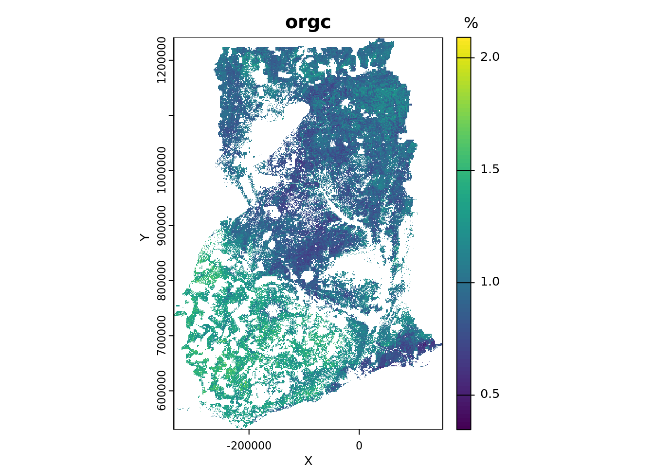

4.5.6 Creating a GeoTIFF layer

Now that we have created a spatial raster object, we can save it as a GIS layer on your computer’s hard disk. We will store the raster in the GeoTIFF format, which is a common and convenient file format for storing raster data. To save a spatial raster object from the terra package, we can use the writeRaster() function. By default, the GeoTIFF will be written with LZW compression.

# save raster to GeoTiff
writeRaster(p_r, filename = tiffFile, overwrite = TRUE)

To save storage space, you might consider converting the unit to $\,\mathrm{g/kg}$ (which is equivalent to multiplying the percentage by 10), and then saving the GeoTiff as an integer file (type = "INT1U") that can store values from 0 to 255. The next code chunk shows how to save the map as a PNG figure in the output/figures folder.

# save raster to png
png(file = pngFile, width = 1200, height = 750, pointsize = 16)
plot(p_r, main = voi, col = terrain.colors(8))
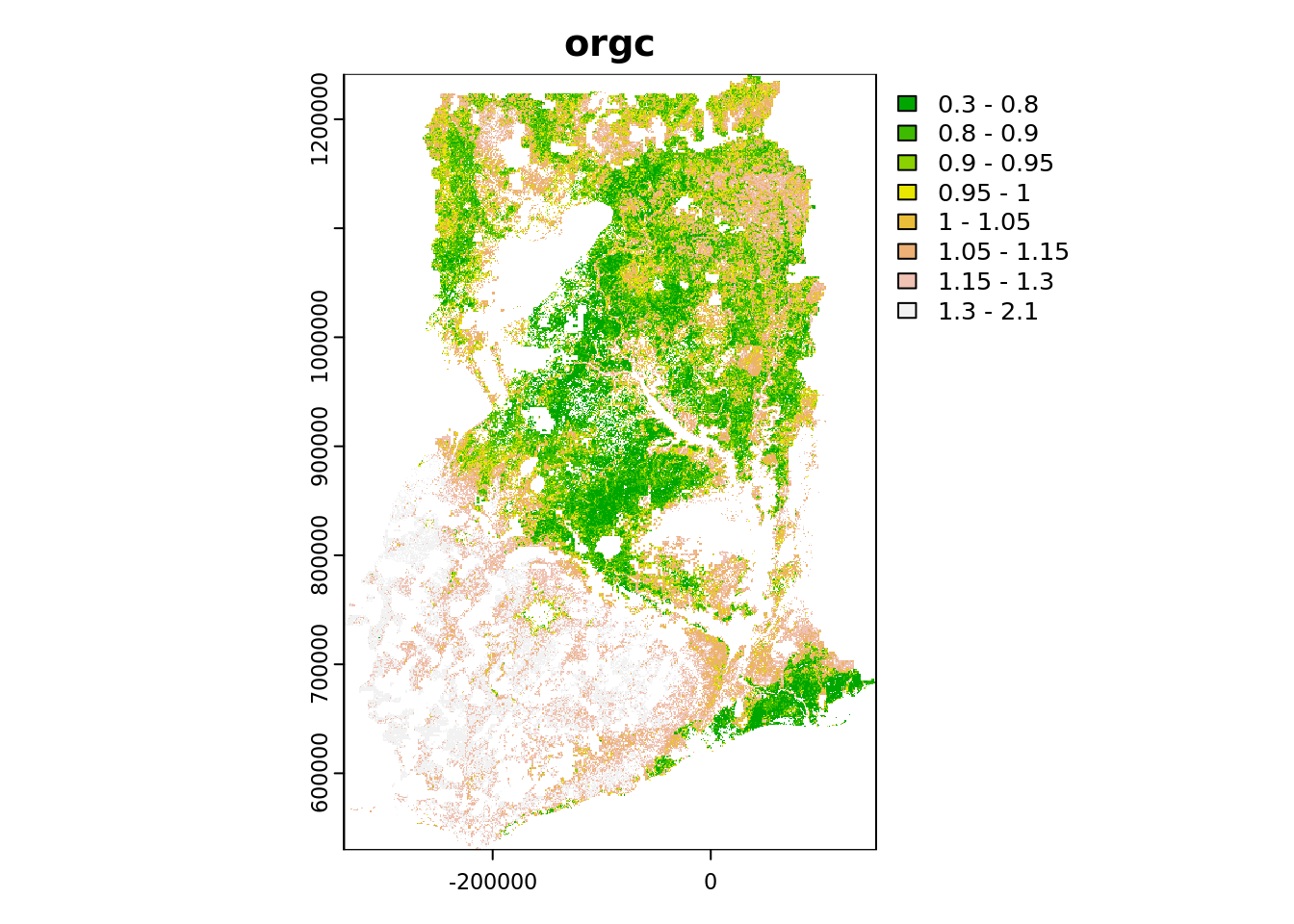
dev.off()

Note that you adjust the color scale of the plot by adding the argument breaks to the plot() function. For instance:

plot(
  p_r,
  breaks = c(0.30, 0.80, 0.90, 0.95, 1.00, 1.05, 1.15, 1.30, 2.10),
  main = voi,
  col = terrain.colors(8)
)

4.5.7 Saving a `terra` raster object

We are now finished and can save the SpatRaster object containing the gridded soil map to the hard disk as an RDS file. Before saving, however, we first need to convert the raster into a packed object, which can be done with the wrap() function of the terra package.

# pack the SpatRaster
p_r <- wrap(p_r)

# check object class
class(p_r)
p_r

# save fitted model to file
saveRDS(p_r, mapFile)

The saved raster object can be read from disk as follows (do not run; example only).

# read RDS file
#p_r <- readRDS(mapFile)

# unpack
#p_r <- rast(p_r)

# Spatial prediction
# end-of-script

4.6 Uncertainty assessment

Traditional random forests produce mean predictions from the ensemble of decision trees, with the mean representing the most likely value given the predictive distribution. Quantile Regression Forests (QRF) is an extension of random forests developed by Nicolai Meinshausen that provides non-parametric estimates of the prediction quantiles, such as the median (50%), 5% and 95%. From these quantiles, spatially explicit, non-parametric estimates of model uncertainty can be derived such as the 90% prediction interval.

This section shows how to:

Section 4.6.3 and Section 4.6.4: Fit a Quantile Random Forest (QRF) model and generate spatial predictions.
Section 4.6.5: Calculate the 90% prediction interval to quantify model uncertainty.
Section 4.6.6: Convert QRF predictions into a spatial raster object.
Section 4.6.7: Saving the gridded maps as a GeoTiff file.
Section 4.6.8: Exporting the resulting terra raster object as an RDS file.

4.6.1 Environment preparation

The following libraries are required for this section:

# load libraries
library(caret)
library(ranger)
library(terra)

We already set the working directory in Chunk 1. It is the same one in which you have saved the outputs from the previous sections.

Our variable of interest (VOI), SOC (%), was defined in Chunk 2.

For this section, we will need to indicate the locations of figures and maps folders as shown in Chunk 4.

We now define objects that contain the file paths to the input data files: in this case the covariate stack, regression matrix and the output of the RFE. Although these objects are used as input in this section, these are all considered outputs of the DSM workflow generated in earlier parts of this manual. As such, these are located in the output directory. We use the file.path() function to create a full file path by combining the output folder path with the respective file names.

# define file paths of the input data
covariateStackFile <- file.path(outputDir,"covariateStack.rds")
regrMatrixFile <- file.path(outputDir, "regressionMatrix.rds")
rfeProfileFile <- file.path(outputDir, paste0("rfeProfile_", voi, ".rds"))

# location and name of the files that will be stored as outputs of this script
mapFile = file.path(outputDir, paste0("rfMap_QRF_", voi, ".rds"))
pngFile = file.path(outputDir_figs, paste0(voi, "_90PI.png"))
tiffFile = file.path(outputDir_maps, paste0(voi, "_90PI.tiff"))

In Chunk 5 we defined the coordinate system of the covariates.

4.6.2 Reading the input data

Start by reading the three required data objects in your R session. These are:

The regression matrix, which includes the training data.
The covariate stack.
The output of the RFE analysis, which contains the selected covariates.

# read regression matrix
rgmx <- readRDS(regrMatrixFile)

# read covariate stack
cs <- readRDS(covariateStackFile)

# read output of RFE
rf_profile <- readRDS(rfeProfileFile)

4.6.3 Fitting a QRF model with ranger

A QRF model can be fitted with the ranger function in much the same way as described in Section 4.2.2 in which a ‘regular’ random forest model was fitted. The only difference is the addition of argument quantreg = TRUE, which enables quantile predictions. As in Section 4.2.2, we start by constructing a model formula. This is done in a single step using a couple of nested functions. For a more detailed explanation of formula construction, refer to Section 4.2.2.

# list names covariates to be used as input and store in new object
covars_rfe <- predictors(rf_profile)

# construct formula string from input soil property and covariate names
mod_for <- as.formula(paste(voi, "~", paste(covars_rfe, collapse = " + ")))

We proceed with fitting a QRF model with the ranger() function.

# fit QRF with ranger
qrf <-
  ranger(
    formula = mod_for,
    data = rgmx,
    quantreg = TRUE,
    importance = "impurity"
  )

4.6.4 Predicting with QRF model

The syntax for making predictions with a QRF mode is very similar to that used in Section 4.5.3. However, in the case of QRF, the type argument must be set to "quantiles", and a vector of desired quantiles must be provided for the quantiles argument. In this manual, we calculate the following quantiles: 0.05, 0.25, 0.5, 0.75, 0.95.

Note that we will predict the median (0.5 quantile), which may differ slightly from the mean prediction obtained by a standard random forest model.

# define quantiles
quants <- c(0.05, 0.25, 0.5, 0.75, 0.95)

# predict with QRF (takes a little while to run)
predQRF <- predict(qrf, data = cs, type = "quantiles", quantiles = quants)

Following the workflow outlined in Section 4.5.3, we compile the predictions into a data.frame and append the corresponding coordinates that can be obtained from the covariate stack.

# compile predictions
pQRF <- data.frame(x = cs$x, y = cs$y, pred = predQRF$predictions)
names(pQRF)

We proceed by assigning more descriptive names to the columns containing the predicted quantiles.

# change column names
names(pQRF)[-(1:2)] <- paste0("Q", quants)
names(pQRF)

# inspect output
head(pQRF)

4.6.5 Calculating the 90% prediction interval

In digital soil mapping, the 90% prediction interval is commonly used to quantify prediction uncertainty. It is calculated as the difference between the 95% and 5% quantile predictions.

# compute 90% prediction interval from 0.95 and 0.05 quantile
pQRF$PI90 <- pQRF[,"Q0.95"] - pQRF[,"Q0.05"]

# inspect results
head(pQRF)

4.6.6 Creating a spatial raster object

The QRF predictions are stored in a data.frame together with their corresponding coordinates. To create a map, we need to convert this data.frame to a spatial raster object, in this case a SpatRaster, which is the raster object class of the terra package.

We can convert a data.frame to a SpatRaster with the rast() function. The process is the same as described in Section 4.5.5; refer to that section for a more detailed explanation.

# convert to a SpatRaster object
pQRF_r <- rast(as.matrix(pQRF), type = "xyz", crs = crs_epsg_covar)

# inspect object
pQRF_r

Now, we will plot the Q05 and Q95 maps to show the quantiles used to compute the 90% prediction interval.To do this, we first need to select the bands of the pQRF_r raster object that correspond to the Q05 and Q95 quantiles.

# store bands of the spatraster object to plot in a new object
bands_plot <- which(names(pQRF_r) %in% c("Q0.05", "Q0.5", "Q0.95"))

Next, determine the value range (i.e., the minimum and maximum) of the quantiles we want to plot. This range is needed to produce appropriate color legends for the plotted maps.

# determine value range for plotting
bands_range <- range(values(pQRF_r[[bands_plot]]), na.rm = TRUE)
bands_range

Plot the maps of the 5% and 95% quantiles.

# save the names of the layers you want to plot
# and the plots titles for each layer
quantiles_plot <- c("Q0.05", "Q0.95")
quantile_main <- c("- 5% quantile", "- 95% quantile")

# plot
for (i in seq_along(quantiles_plot)){
  plot(pQRF_r[[quantiles_plot[i]]], 
       range = bands_range,
       main = paste(voi, quantile_main[i]),
       xlab = "X", ylab = "Y", 
       plg = list(title = "%"))
}

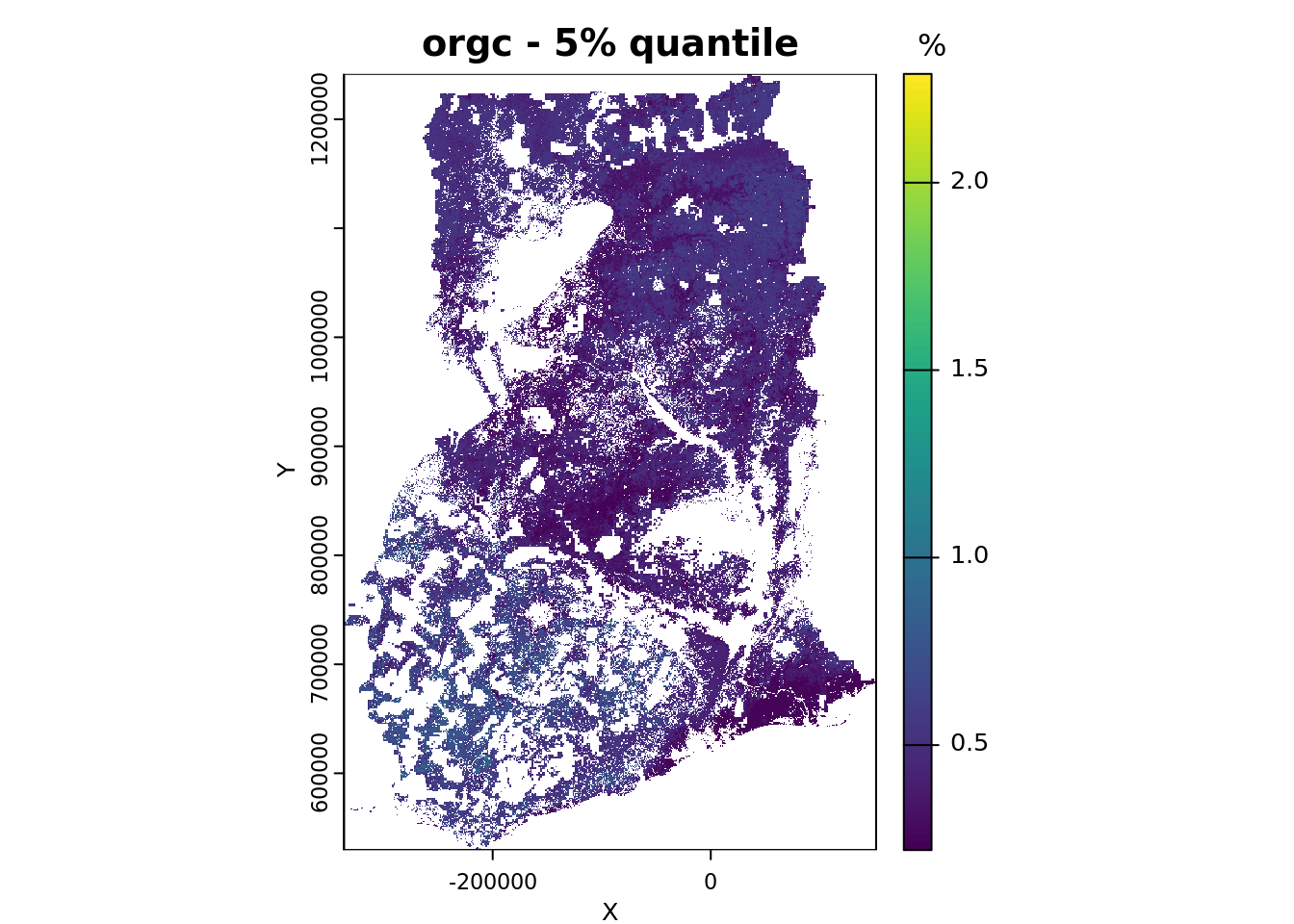
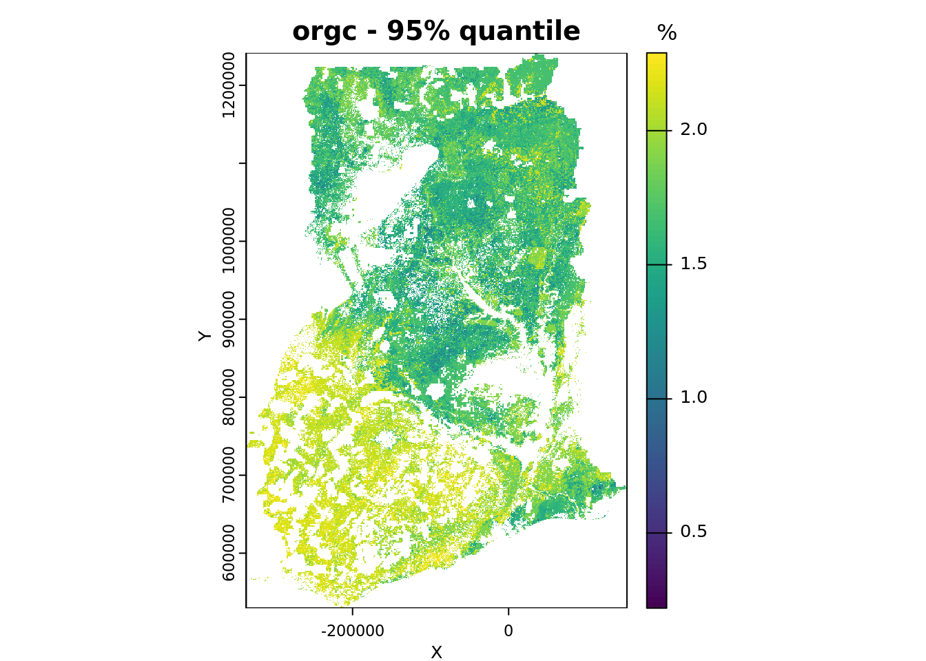
We conclude by plotting the map showing the width of the 90% prediction interval. We use a different color ramp for this purpose.

plot(pQRF_r[["PI90"]], 
     col = heat.colors(64),
     main = paste(voi, "- 90% Prediction interval width"))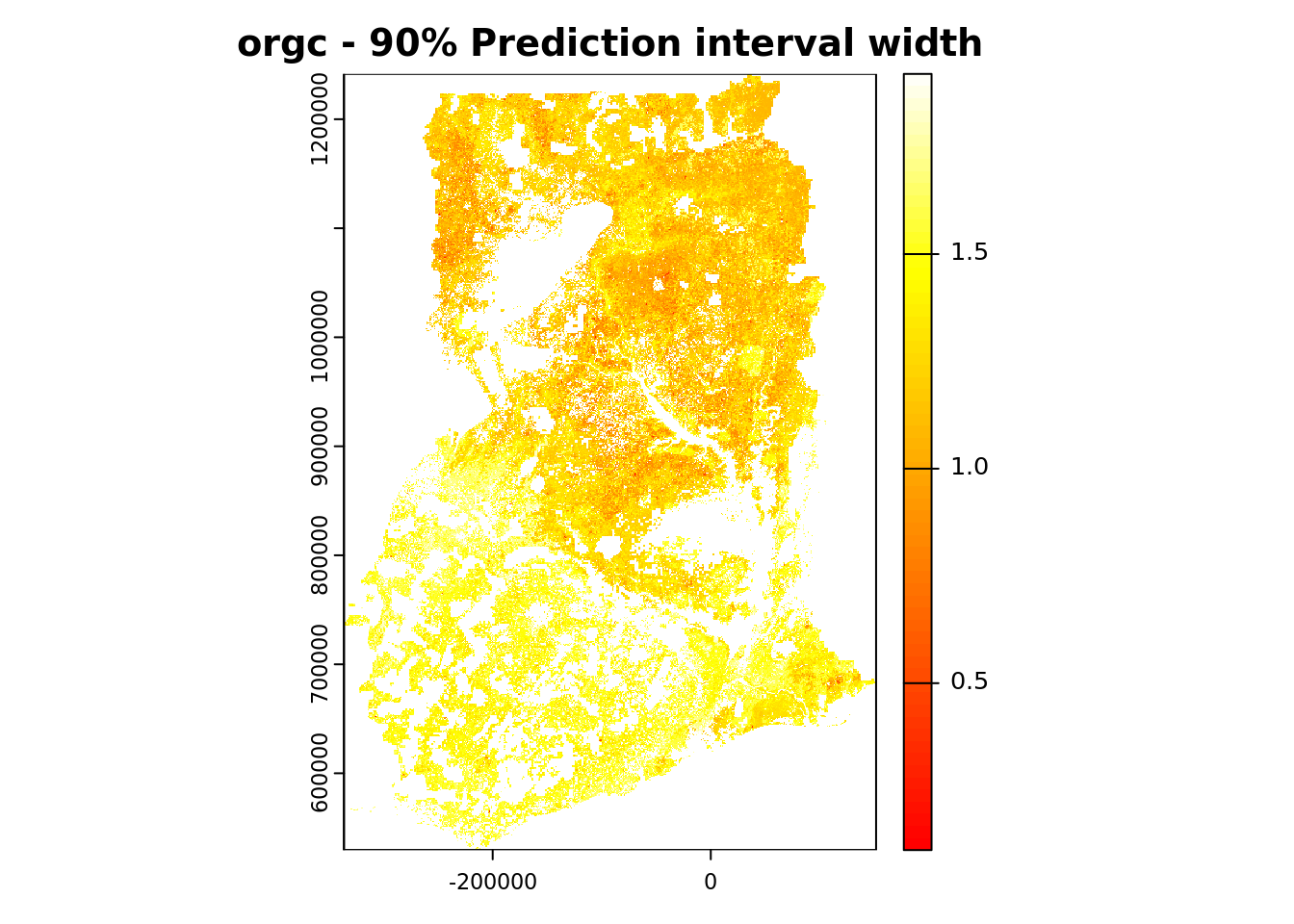

Absolute uncertainty is lower in areas with low predicted values and higher in areas with high predicted values (compare with the map produced in Section 4.5.5).

4.6.7 Creating a GeoTIFF layer

Now that we have created a spatial raster object, we can save it as a GIS layer on the hard disk. We store the raster in GeoTIFF format. Saving a spatial raster object from the terra package can be done with the writeRaster() function. The GeoTIFF is written with LZW compression by default. Here we save the 90% prediction interval grid.

# save raster to GeoTiff
writeRaster(pQRF_r[["PI90"]], filename = tiffFile, overwrite = TRUE)

The next code chunk shows how to save the 90% prediction interval grid as a PNG figure (in the output/figures folder).

# save raster to png
png(file = pngFile, width = 1200, height = 750, pointsize = 16)
plot(pQRF_r[["PI90"]], main = paste(voi, "- 90% prediction interval width"), col = terrain.colors(8))
dev.off()

4.6.8 Saving a `terra` raster object

We are done and can now save the SpatRaster object containing the quantile layers to disk as an RDS file. Before saving, we first convert the raster into a packed object using the wrap() function of the terra package.

# pack the SpatRaster
pQRF_r <- wrap(pQRF_r)

# check object class
class(pQRF_r)
pQRF_r

# save fitted model to file
saveRDS(pQRF_r, mapFile)

The saved raster object can be loaded from disk as shown below (uncomment the lines to run it, if needed).

# read RDS file
#pQRF_r <- readRDS(mapFile)

# unpack
#pQRF_r <- rast(pQRF_r)

# Uncertainty assessment
# end-of-script

4.1 Set up

4.2 Model fitting

4.2.1 Reading the regression matrix

4.2.2 Fitting a random forest model

4.2.3 Inspecting model output and variable importance

4.3 Recursive Feature Elimination (RFE)

4.3.1 Environment preparation

4.3.2 Read data and prepare RFE inputs

4.3.3 Run RFE and inspect results

4.3.4 Fit RF model based on RFE outcome

4.4 Accuracy assessment

4.4.1 Environment preparation

4.4.2 Read data

4.4.3 Accessing accuracy statistics

4.4.4 Accessing accuracy statistics after RFE

4.4.5 Compiling accuracy statistics

4.5 Spatial prediction

4.5.1 Environment preparation

4.5.2 Read the input data

4.5.3 Predict the soil property of interest

4.5.4 Compiling the predictions

4.5.5 Creating a spatial raster object

4.5.6 Creating a GeoTIFF layer

4.5.7 Saving a terra raster object

4.6 Uncertainty assessment

4.6.1 Environment preparation

4.6.2 Reading the input data

4.6.3 Fitting a QRF model with ranger

4.6.4 Predicting with QRF model

4.6.5 Calculating the 90% prediction interval

4.6.6 Creating a spatial raster object

4.6.7 Creating a GeoTIFF layer

4.6.8 Saving a terra raster object

4.5.7 Saving a `terra` raster object

4.6.8 Saving a `terra` raster object