# Empty memory and workspace
gc()
rm(list = ls())

# Modify this file path with the location where you saved the tutorial files
workingDir <- file.path("C:/soil_water_nutrients")

# Set up working directories
setwd(workingDir)
scripts_path <- file.path(workingDir, "code/functions")
filesDir <- file.path(workingDir, "soil-water")2 Plant-available soil water
Required libraries and external functions for this section:
# Load libraries
require(terra)
require(knitr)

# Call external functions
source(file.path(scripts_path, "VMCPTF_function.R"))
source(file.path(scripts_path, "EffPAWHC_function.R"))
source(file.path(scripts_path, "Auxiliary_functions.R"))
2.1 Input data for assessing root zone plant-available soil water holding capacity
This section reads the input data (maps) required to calculate root zone plant-available soil water holding capacity (RZ-PAWHC) according to the procedure described by Leenaars et al., 2018. These data will be used in Section 2.2 to calculate the effective plant-available water holding capacity of soil depth intervals, and in Section 2.3 to calculate rootable depth and the effective plant-available water holding capacity of the rootable depth.
In this section required soil property maps of the targeted area are read in and explored.
Africa soilgrids data available per depth interval and required as input data to the external functions (6 values for 6 depth intervals per pixel):
LayerNr = number of standard depth interval (sd1-sd6; 0-5, 5-15, 15-30, 30-60, 60-100, 100-200 cm)
- UpDpth = upper horizon depth (cm)
- LowDpth = lower horizon depth (cm)
- CrsFrg = volumetric coarse fragments content (m3/100m3)
- Sand = sand fraction (g/100g)
- Silt = silt fraction (g/100g)
- Clay = clay fraction (g/100g)
- BulkDens = bulk density of the fine earth fraction * 1000 (kg/m3)
- pHH2O = pHH2O * 10
- EC = electric conductivity (dS/m)
- CEC = cation exchange capacity (cmolc/kg)
- ExchNa = exchangeable Na content (cmolc/kg)
- ExchBases = exchangeable bases (cmolc/kg)
- ExchAcids = exchangeable acidity (cmolc/kg)
- CaSO4 = gypsum content (g/kg); not available
- CaCO3 = carbonate equivalent (g/kg); not available
- OrgC = organic C content (g/kg)
## Read input maps for the functions
maps.lst <- c("Sand", "Silt", "Clay", "CrsFrg", "OrgC",
              "BulkDens", "CEC", "pHH2O", "ExchBases",
              "EC", "ExchAcids", "ExchNa")

#all the input raster layers are read using this loop
for (i in 1:length(maps.lst)){
  assign(maps.lst[i], rast(paste0(filesDir, "/", maps.lst[i],
                                  c("_sd1.tif", "_sd2.tif", "_sd3.tif",
                                    "_sd4.tif", "_sd5.tif", "_sd6.tif"))))
} # One stack is created per property

# for example, 6 raster maps for sand are stored in one stack
# during the practical we will select the stacks for the needed
# properties and the needed depth intervals from these stacks
Sand
# this is the selection of the second layer (depth interval) for Sand
Sand[[2]]
We need to know the upper and lower depths of each of the raster maps (of each of the standard depth intervals).
sd1in the file name means 0 - 5 cmsd2in the file name means 5 - 15 cmsd3in the file name means 15 - 30 cmsd4in the file name means 30 - 60 cmsd5in the file name means 60 - 100 cmsd6in the file name means 100 - 200 cm
# create a vector object containing the interval depth for each of the layers
UpDpth <- c(0, 5, 15, 30, 60, 100)
LowDpth <- c(5, 15, 30, 60, 100, 200)
We’ll now show maps and summary statistics for each soil property and each depth interval using the customized function stats.all.
for (i in seq_along(maps.lst)) {
print(kable(stats.all(get(maps.lst[i]))))
print(maps.lst[i])
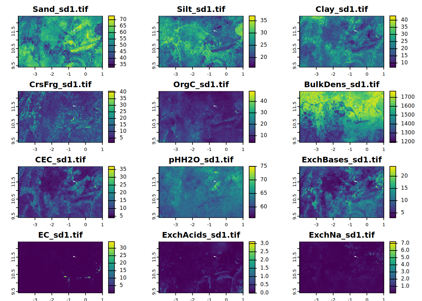
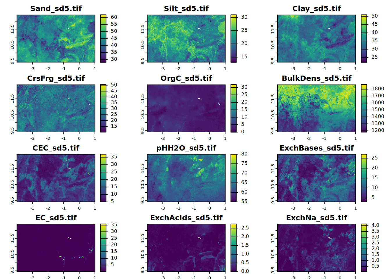
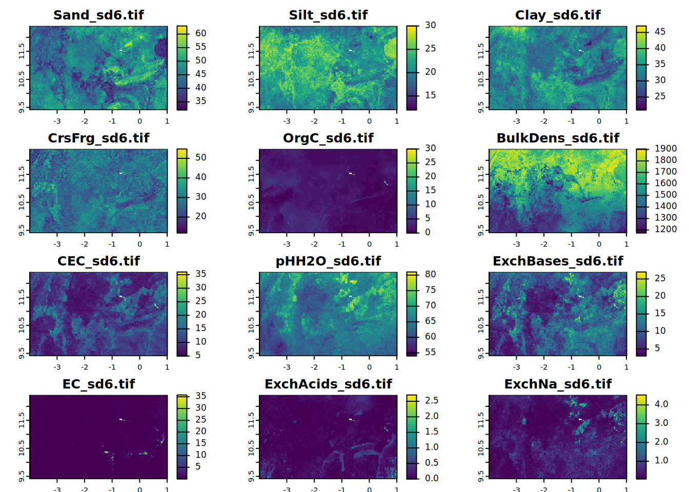
}The soil property data by depth interval can be plotted with the terra::plot function. Use the following code to map and view soil property data for specific depth intervals. The graphs are organized in a 4x3 matrix using par(), which sets or queries graphical parameters. The terra::summary function can also print per-layer summary statistics of a raster stack.
## Explore the soil input data per layer

# list the rasters
all.properties.sd <- list(Sand, Silt, Clay, CrsFrg, OrgC,
                          BulkDens, CEC, pHH2O, ExchBases,
                          EC, ExchAcids, ExchNa)

# map visualization of soil property data for a specific sd
# Create a 4 rows x 3 columns plotting matrix
par(mfrow = c(4, 3))

# sd1
for (i in seq_along(all.properties.sd)){
  plot(all.properties.sd[[i]][[1]],
       main = paste0(maps.lst[i], "_sd1.tif"),
       mar = c(1, 1.5, 2, 4)) # mar = c(bottom, left, top and right)
}
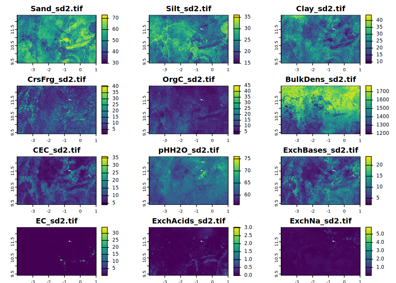
# sd2
for (i in seq_along(all.properties.sd)){
  plot(all.properties.sd[[i]][[2]],
       main = paste0(maps.lst[i], "_sd2.tif"),
       mar = c(1, 1.5, 2, 4))
}
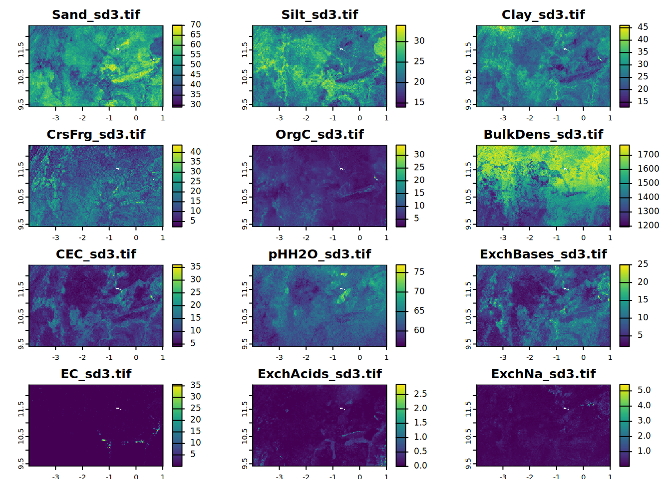
# sd3
for (i in seq_along(all.properties.sd)){
  plot(all.properties.sd[[i]][[3]],
       main = paste0(maps.lst[i], "_sd3.tif"),
       mar = c(1, 1.5, 2, 4))
}
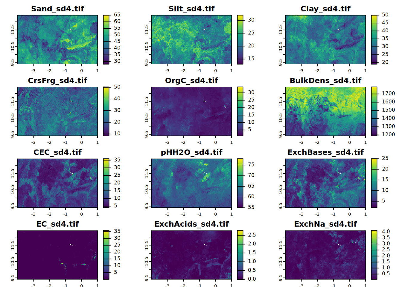
# sd4
for (i in seq_along(all.properties.sd)){
  plot(all.properties.sd[[i]][[4]],
       main = paste0(maps.lst[i], "_sd4.tif"),
       mar = c(1, 1.5, 2, 4))
}
# sd5
for (i in seq_along(all.properties.sd)){
  plot(all.properties.sd[[i]][[5]],
       main = paste0(maps.lst[i], "_sd5.tif"),
       mar = c(1, 1.5, 2, 4))
}
# sd6
for (i in seq_along(all.properties.sd)){
  plot(all.properties.sd[[i]][[6]],
       main = paste0(maps.lst[i], "_sd6.tif"),
       mar = c(1, 1.5, 2, 4))
}
# print summary statistics
summary(Sand)
2.1.1 Explore the Africa SoilGrids input data
Africa SoilGrids data available for the profile as a whole and required as input data to the external functions (1 value per pixel):
- Mask = Gaul land mask
# We will use the pHH2O[[1]] map as 'dummy' object, then a constant (1)
# is assigned to all the pixels of the area of interest.
mask <- pHH2O[[1]] # this is a dummy variable
mask <- ifel(is.na(mask), NA, 1)- drainClasses =
- very poorly
- poorly
- imperfectly
- moderately well
- well
- somewhat excessively
- excessively drained
- RockDpth = depth (cm) to bedrock (R) or an iron pan (Bmc)
- CropDpth = 150 cm (maximum rooting depth of the considered crop; Maize)
# create a new raster with a constant value
CropDpth <- mask * 150
# read the depth to bedrock map
RockDpth <- rast(file.path(filesDir, "RockDpth.tif"))
# read the drain classes map
drainClasses <- rast(file.path(filesDir, "drainClasses.tif"))

plot(drainClasses, main = "drainClasses", mar = c(1.2, 0.5, 1.5, 1))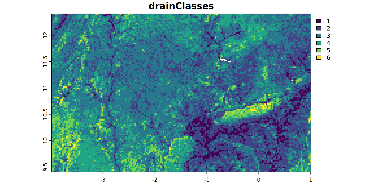
summary <- freq(drainClasses, digits = 0)
kable(summary[, 2:3])
summary <- stats.all(drainClasses)
kable(summary)plot(RockDpth, main = "RockDpth", mar = c(1.2, 0.5, 1.5, 1))
summary <- stats.all(RockDpth)
kable(summary)
2.2 Effective plant-available soil water holding capacity per depth interval
We’ll first derive and map soil water retention (volumetric moisture content) per depth interval, at predefined tensions, using a pedotransfer function. Required soil property data includes sand, silt, clay, bulk density, pHH2O, CEC and organic carbon.
Now let’s prepare the data for being used in the pedotransfer function.
# pHH2O values are multiplied per 10; here we divide pHH2O by 10
pHH2O <- pHH2O / 10

# fix texture values
sum.tex <- Clay + Silt + Sand
Clay <- Clay / (sum.tex) * 100
Silt <- Silt / (sum.tex) * 100
Sand <- Sand / (sum.tex) * 100
sum.tex <- Clay + Silt + Sand
Then property data are ready to use the VMCPTF function.
Next steps is to calculate volumetric moisture content (VMC; 0-1 m3/m3) of the soil fine earth fraction for each depth interval at the following tensions (suction pressures, hydraulic heads):
- saturation (tetaS), defined as h0 = 1 cm (= -0.1 kPa = -0.001 bar = pF 0.0)
- field capacity (FC), defined as h1 = 100 cm (= -10 kPa = 0.1 bar = pF 2.0)
- field capacity (FC), defined as h2 = 200 cm (= -20 kPa = 0.2 bar = pF 2.3)
- field capacity (FC), defined as h3 = 300 cm (= -30 kPa = 0.3 bar = pF 2.5): defined here as h3 = 316 cm
- permanent wilting point (PWP), defined as h4 = 15.850 cm (= -1585 kPa = -16 bar = pF 4.2)
# create an empty list to store the results per interval depth
VMCPTF <- list(NULL)

for (x in 1:6) { # loop to apply the function to 6 depths

  # stack all the input data needed for the same layer depth
  input <- c(Sand[[x]], Silt[[x]], Clay[[x]], OrgC[[x]],
             BulkDens[[x]], CEC[[x]], pHH2O[[x]], CrsFrg[[x]],
             ExchBases[[x]], EC[[x]], ExchAcids[[x]])

  # adapt the names of the raster compiled layers
  names(input) <- c("Sand", "Silt", "Clay", "OrgC", "BulkDens", "CEC",
                    "pHH2O", "CrsFrg", "ExchBases", "EC", "ExchAcids")

  # apply the function VMCPTF.function
  VMCPTF[[x]] <- VMCPTF.function(Sand = input[["Sand"]],
                                 Silt = input[["Silt"]],
                                 Clay = input[["Clay"]],
                                 OrgC = input[["OrgC"]],
                                 BulkDens = input[["BulkDens"]],
                                 CEC = input[["CEC"]],
                                 pHH2O = input[["pHH2O"]],
                                 h1 = -10, h2 = -20,
                                 h3 = -31.6, h4 = -1585,
                                 PTF.coef, fix.values = TRUE,
                                 print.coef = TRUE)

} # h0 is defined and then VMC_h0 is calculated in the function
You can explore the function main steps. Open the VMCPTF_funtion.R script (in the _functions folder) and try to understand the different steps. Also let’s explore the results after aplying the VMCPTF.function:
- Statistics for VMC-h0
VMC_h0 <- lapply(VMCPTF, function(l) l[[1]])
VMC_h0 <- do.call(c, VMC_h0)
summary <- stats(VMC_h0, 6)
kable(summary)- Statistics for VMC-h1
VMC_h1 <- lapply(VMCPTF, function(l) l[[2]])
VMC_h1 <- do.call(c, VMC_h1)
summary <- stats(VMC_h1, 6)
kable(summary)- Statistics for VMC-h2
VMC_h2 <- lapply(VMCPTF, function(l) l[[3]])
VMC_h2 <- do.call(c, VMC_h2)
summary <- stats(VMC_h2, 6)
kable(summary)- Statistics for VMC-h3
VMC_h3 <- lapply(VMCPTF, function(l) l[[4]])
VMC_h3 <- do.call(c, VMC_h3)
summary <- stats(VMC_h3, 6)
kable(summary)- Statistics for VMC-h4
VMC_h4 <- lapply(VMCPTF, function(l) l[[5]])
VMC_h4 <- do.call(c, VMC_h4)
summary <- stats(VMC_h4, 6)
kable(summary)
You can also visualize the resulting maps with below code.
# VMC at saturation
plot(VMC_h0, mar = c(1, 1.5, 2, 4),
     main = c("VMC_h0_sd1", "VMC_h0_sd2", "VMC_h0_sd3",
              "VMC_h0_sd4", "VMC_h0_sd5", "VMC_h0_sd6"))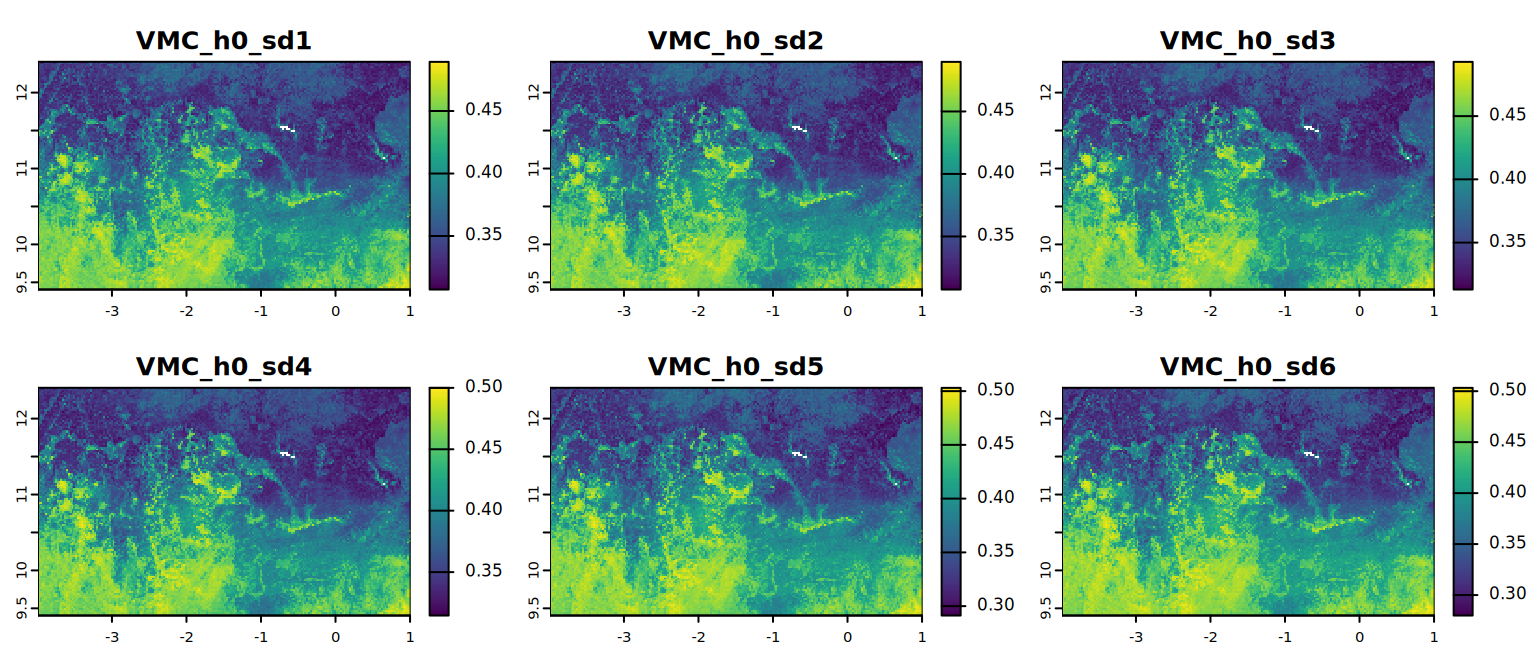
# VMC at field capacity (default)
plot(VMC_h1, mar = c(1, 1.5, 2, 4),
     main = c("VMC_h1_sd1", "VMC_h1_sd2", "VMC_h1_sd3",
              "VMC_h1_sd4", "VMC_h1_sd5", "VMC_h1_sd6"))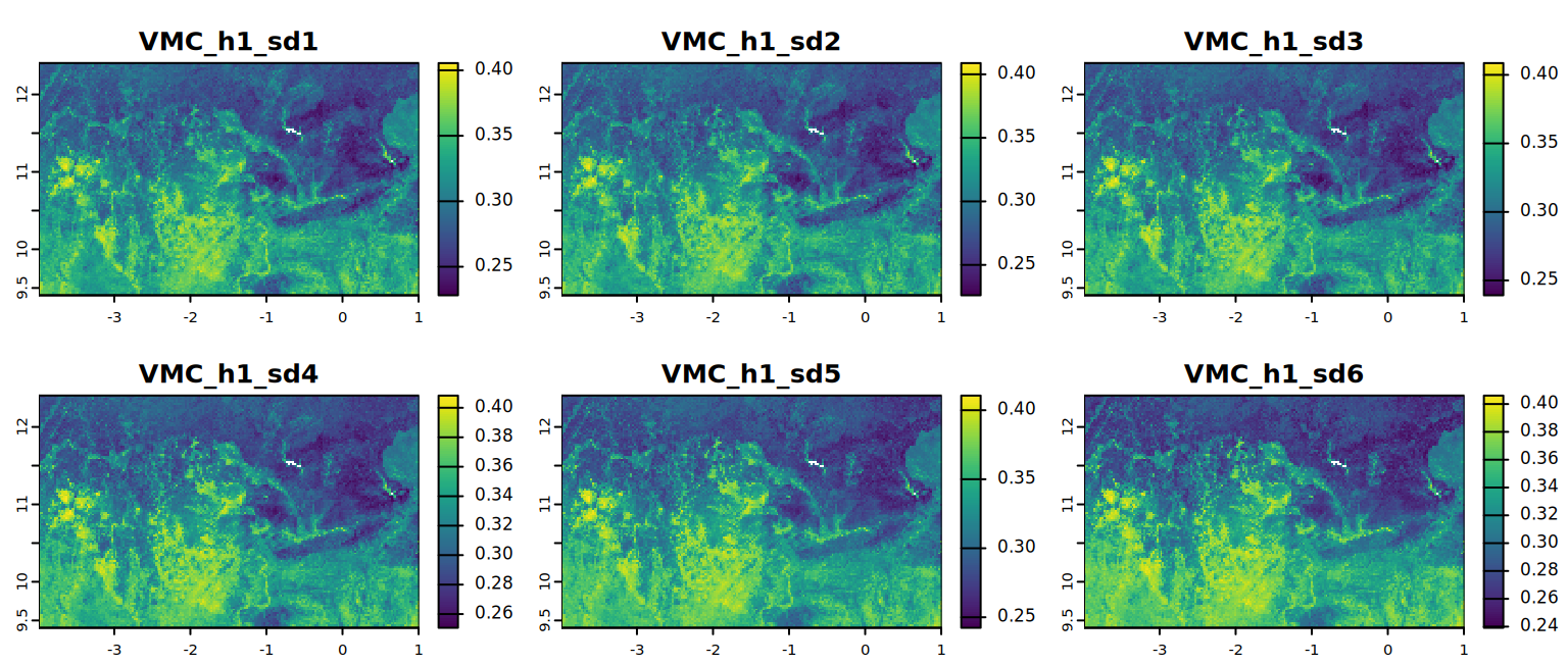
# VMC at field capacity (alternative)
plot(VMC_h2, mar = c(1, 1.5, 2, 4),
     main = c("VMC_h2_sd1", "VMC_h2_sd2", "VMC_h2_sd3",
              "VMC_h2_sd4", "VMC_h2_sd5", "VMC_h2_sd6"))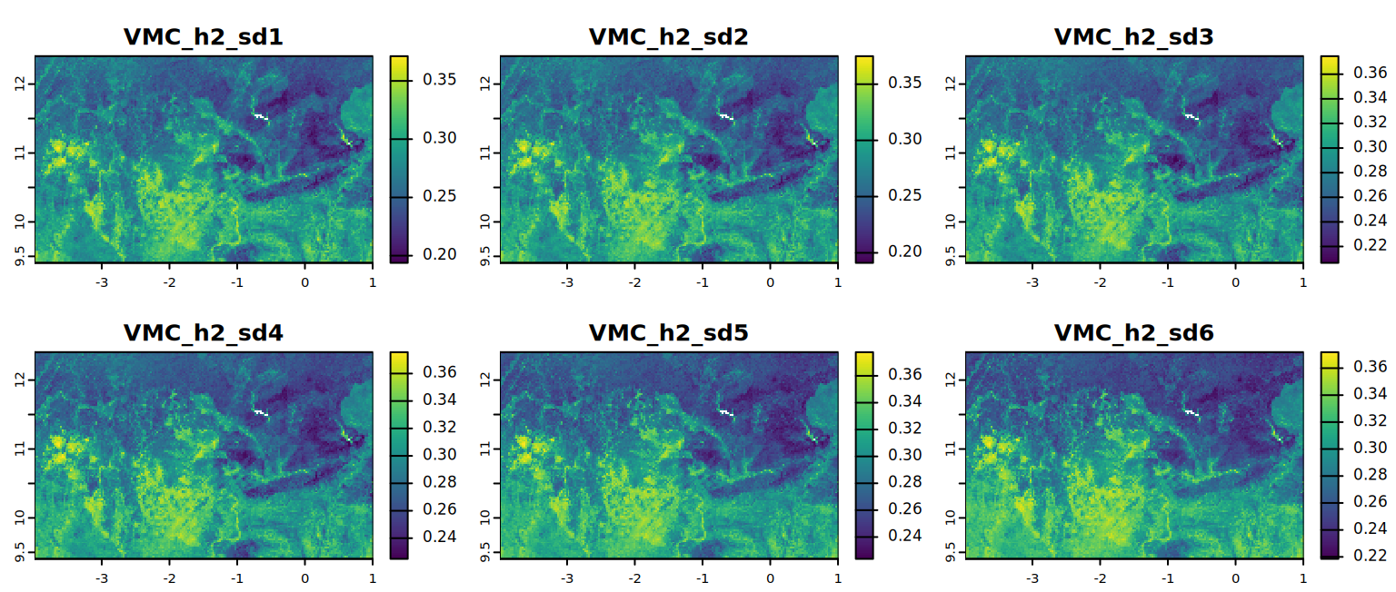
# VMC at field capacity (alternat)
plot(VMC_h3, mar = c(1, 1.5, 2, 4),
     main = c("VMC_h3_sd1", "VMC_h3_sd2", "VMC_h3_sd3",
              "VMC_h3_sd4", "VMC_h3_sd5", "VMC_h3_sd6"))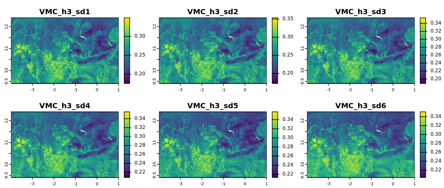
# VMC at permanent wilting point
plot(VMC_h4, mar = c(1, 1.5, 2, 4),
     main = c("VMC_h4_sd1", "VMC_h4_sd2", "VMC_h4_sd3",
              "VMC_h4_sd4", "VMC_h4_sd5", "VMC_h4_sd6"))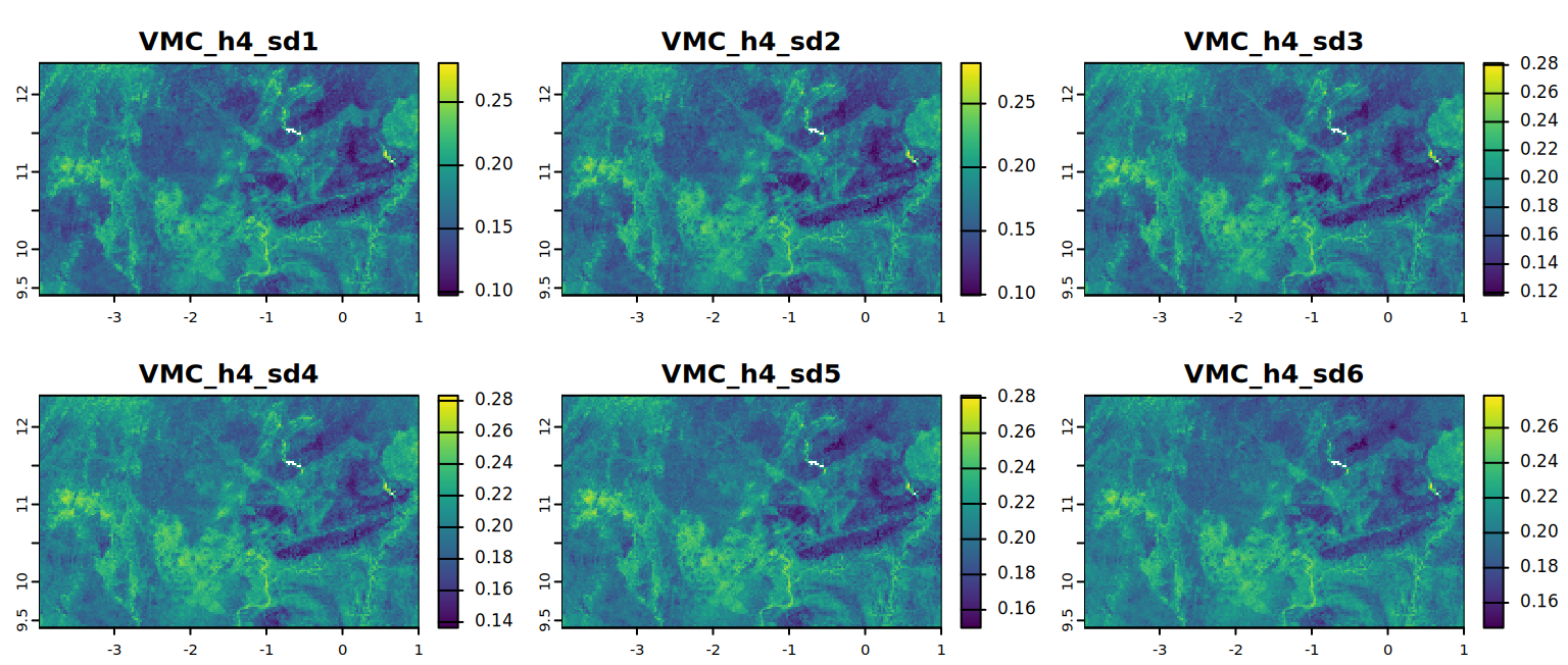
Next step is to calculate plant-available water holding capacity (PAWHC; 0-1 m3/m3) for each depth interval with field capacity (FC) defined as 100 cm (h1). PAWHC = VMC at FC (h1) minus VMC at PWP (h4).
# create an empty list to store the results per interval depth
PAWHC.sd <- list(NULL)

for (x in 1:6) { # loop to apply the function to 6 depths

PAWHC.sd[[x]] <- PAWHC.function(LowDpth[x], UpDpth[x],
                                VMCPTF[[x]]$VMC_h1,
                                VMCPTF[[x]]$VMC_h4)
names(PAWHC.sd[[x]]) <- c("PAWHC", "PAWHC_mm")
}
# note that this object is a list with 6 elements (one per depth interval).
#Each list  stores 2 variables calculated. In this case PAWHC, PAWHC_mm.
Explore statistics and maps for PAWHC per sd (std depth interval) produced in the last step.
PAWHC <- lapply(PAWHC.sd, function(l) l[[1]])
PAWHC <- do.call(c, PAWHC)
summary <- stats(PAWHC, 6)
kable(summary)plot(PAWHC, mar = c(1, 1.5, 2, 4),
main = c("PAWHC_sd1", "PAWHC_sd2", "PAWHC_sd3",
"PAWHC_sd4", "PAWHC_sd5", "PAWHC_sd6"))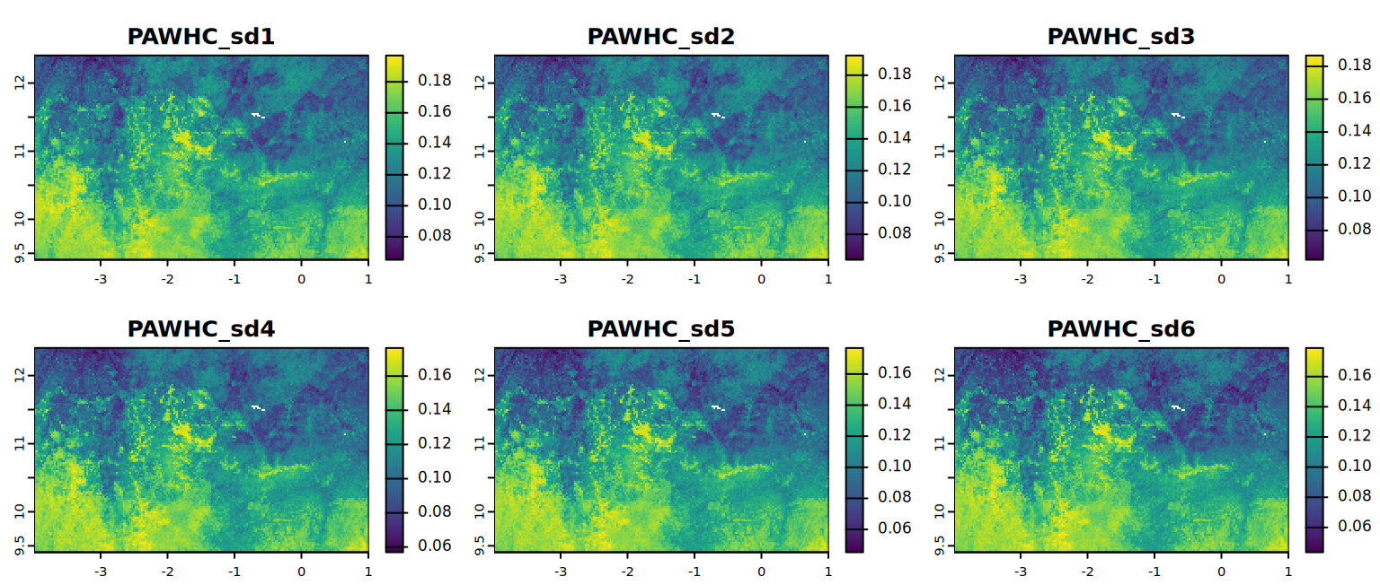
Also calculate effective PAWHC (EffPAWHC; 0-1 m3/m3) of the soil whole earth for each depth interval (effective is considering volumetric coarse fragments content).
# create an empty list to store the results per interval depth
EffPAWHC.sd <- list(NULL)

for (x in 1:6) { # loop to apply the function to 6 depths

 EffPAWHC.sd[[x]] <- EffPAWHC.function(LowDpth[x], UpDpth[x],
                                       CrsFrg = CrsFrg[[x]],
                                       PAWHC = PAWHC[[x]]$PAWHC)

} # note that this object is a list with 6 elements (one per depth interval)
# Each list  stores 3 variables calculated
# In this case PAWHC, EffPAWHC, EffPAWHC_mm. Why again PAWHC?
Explore the statistics for EffPAWHC per sd (std depth interval) calculated in the last step.
# Results for layer sd1
EffPAWHC <- lapply(EffPAWHC.sd, function(l) l[[2]])
EffPAWHC <- do.call(c, EffPAWHC)
summary <- stats(EffPAWHC, 6)
kable(summary)plot(EffPAWHC, mar = c(1, 1.5, 2, 4),
main = c("EffPAWHC_sd1", "EffPAWHC_sd2",
"EffPAWHC_sd3", "EffPAWHC_sd4",
"EffPAWHC_sd5", "EffPAWHC_sd6"))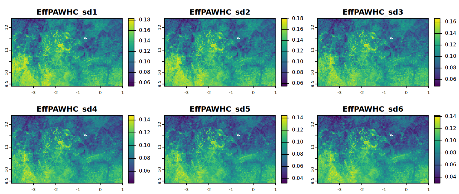
As final steps for this section, now calculate the total PAWHC (TPAWHC_mm) and total effective PAWHC (EffTPAWHC_mm) of the soil aggregated over 0-150 cm. This the absolute quantity of plant-available water (in mm) that the soil can hold within 150 cm. We also calculate the total average PAWHC and EffPAWHC (TPAWHC and EffTPAWHC in m3/m3).
- Calculate the total average PAWHC in 0-150 cm depth (TPAWHC in m3/m3).
# calculate average TPAWHC till 150 cm
TPAWHC <- (PAWHC[[1]] * 5 + PAWHC[[2]] * 10 + PAWHC[[3]] * 15 +
PAWHC[[4]] * 30 + PAWHC[[5]] * 40 + PAWHC[[6]] * 100 / 2) / 150- Calculate the total average EffPAWHC in 0-150 cm depth (EffTPAWHC in m3/m3)
# calculate EffTPAWHC till 150 cm
EffTPAWHC <- (EffPAWHC[[1]] * 5 + EffPAWHC[[2]]*10 +  EffPAWHC[[3]] * 15 +
                EffPAWHC[[4]] * 30 + EffPAWHC[[5]] * 40 +
EffPAWHC[[6]] * 100 / 2) / 150- Calculate the total absolute PAWHC in 0-150 cm depth (TPAWHC_mm in mm)
# extract PAWHC from PAWHC.sd object
PAWHC_mm <- lapply(PAWHC.sd, function(l) l[[2]])
PAWHC_mm <- do.call(c, PAWHC_mm)
# calculation
TPAWHC_mm <- PAWHC_mm[[1]] + PAWHC_mm[[2]] + PAWHC_mm[[3]] +
PAWHC_mm[[4]] + PAWHC_mm[[5]] + PAWHC_mm[[6]] / 2- Calculate the total absolute EffPAWHC in 0-150 cm depth (EffTPAWHC_mm in mm)
# extract EffPAWHC from EffPAWHC object
EffPAWHC_mm <- lapply(EffPAWHC.sd, function(l) l[[3]])
EffPAWHC_mm <- do.call(c, EffPAWHC_mm)
# calculation
EffTPAWHC_mm <- EffPAWHC_mm[[1]] + EffPAWHC_mm[[2]] +  EffPAWHC_mm[[3]] +
  EffPAWHC_mm[[4]]  + EffPAWHC_mm[[5]]  +   EffPAWHC_mm[[6]] / 2
See and interpret the summary statistics and maps for TPAWHC_mm and EffTPAWHC_mm.
plot(TPAWHC_mm, main = "TPAWHC_mm", mar = c(1.2, 0.5, 1.5, 1))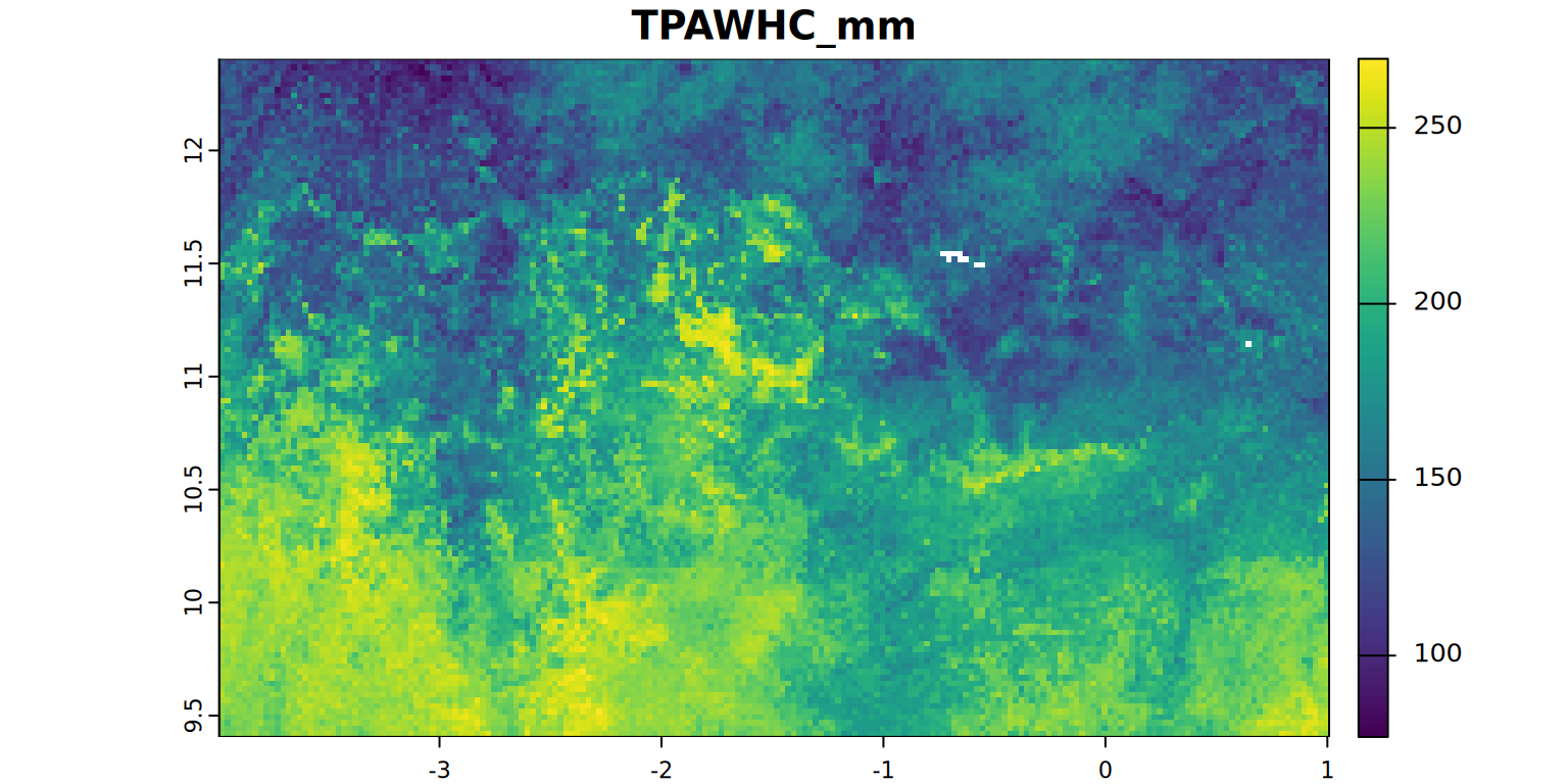
# summary statistics of the data for the selected property
summary <- stats(TPAWHC_mm, 1)
kable(summary)plot(EffTPAWHC_mm, main = "EffTPAWHC_mm", mar = c(1.2, 0.5, 1.5, 1))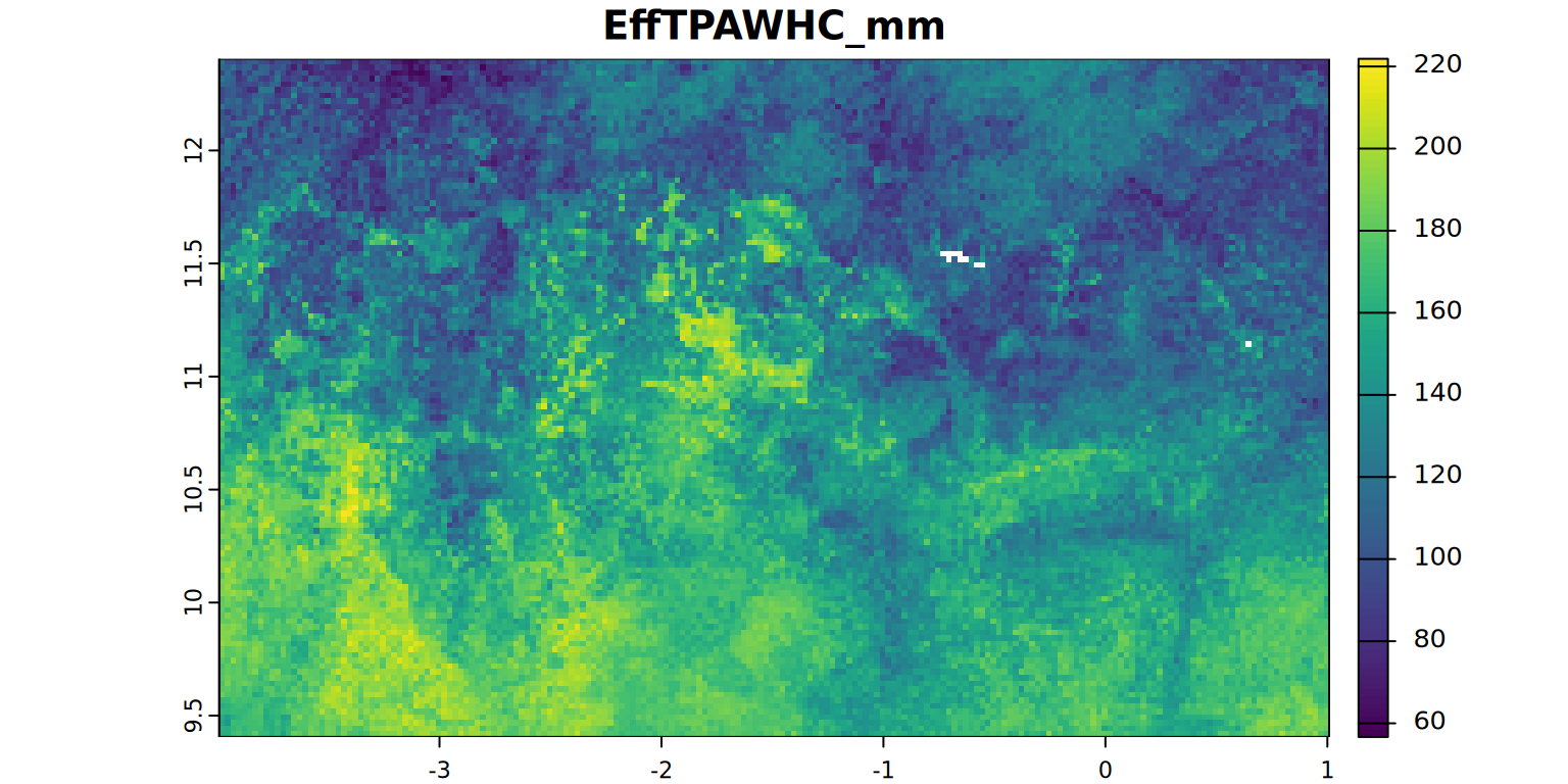
# summary statistics of the data for the selected property
summary <- stats(EffTPAWHC_mm, 1)
kable(summary)
2.3 Mapping soil rootable depth and root zone plant-available water holding capacity
In this section:
We’ll calculate and map the soil rootable depth, also called the effective root zone depth (RZD), for maize and then the root zone plant-available water holding capacity.
We’ll use the inference rules developed for the Global Yield Gap Atlas (GYGA) project; See Leenaars et al. (2018).
Required soil property data (already read) are:
- Data per depth interval (6 values per pixel): UpDpth, LowDpth, CrsFrg, Sand, Silt, Clay, BulkDens, pHH2O, EC, CEC, ExchNa, ExchBases, ExchAcids, CaSO4, CaCO3, OrgC, VMC_h0 (note that VMC_h0 was calculated in the above VMCPTF_function).
- Data for the soil profile as a whole (1 value per pixel): DrainClasses, RockDpth.
- Soil factors, or soil qualities, are derived from these soil properties and the derived values are evaluated to calculate factor-specific rootable depths. These depths are compared to conclude the shallowest one being the soil rootable depth.
Soil factors evaluated for each of the 6 depth intervals (with the variable name indicated between brackets) are :
- adequacy of soil volume (CrsFrg),
- porosity (VMC_h0 and BulkDens,f); f considers clay content,
- adequacy of soil texture (Sand),
- abruptness of soil textural change (Sand.d, Clay.d); d considers distance in cm,
- acidity (pHH2O.L),
- alkalinity (pHH2O.H),
- salinity (EC),
- sodicity (ExchNa, ExchNa.f); f considers CEC,
- toxicity (ExchAcids, ExchAcids.f); f considers CEC,
- cementation (CaCO3, CaSO4). Note that CaCO3 and CaSO4 are named CRB and GYP in the remainder of the text.
Soil factors evaluated for the soil profile as a whole are :
- depth of soil to oxygen shortage (drainDpth),
- depth of soil to bedrock or indurated iron pan (rockDpth)
- depth of soil to where the considered crop (Maize) is genetically able to root without soil restrictions (cropDpth)
See Leenaars et al., 2018 for details on how the soil factor values are derived from the soil property values.
First we call the required external functions.
source(file.path(scripts_path, "RI_function.R"))
source(file.path(scripts_path, "EvaluateRI_function.R"))
source(file.path(scripts_path, "Spline_function.R"))
The derived values for the soil factors per depth interval are evaluated through rootability indices (0-100%). The criteria are given here indicating the factor values corresponding with 100% rootability (ERscore1) and 0% rootability (ERscore2).
A threshold index (Score) is defined for each of the factor-specific rootability indices beyond (below) which the rootability is considered fully constrained (RI=0%) and above which fully unconstrained (RI=100%). These threshold indices are set at 25% by default but can be adjusted for each factor separately.
Default threshols are defined below.
# you can adjust the thresholds by creating a new object
# called "thresholds" and then changing the scores
rn <- c("range", "CrsFrg", "VMC_h0", "BulkDens.f", "Sand", "Clay.d",
        "Sand.d", "pHH2O.L", "pHH2O.H", "EC", "ExchNa.f", "ExchNa",
        "ExchAcids.f", "ExchAcids", "CRB", "GYP")

thresholds <- data.frame(
  ERscore1 = c(100, 80, 50, 0, 95, 40, 40, 5.5, 7.8,
               1.5, 10, 1, 35, 2.5, 150, 150),
  ERscore2 = c(0, 90, 30, 0.35, 100, 60, 60, 4, 9.05,
               6.75, 25, 5, 85, 6.5, 750, 750),
  Trend = c(0, -1, 1, -1, -1, -1, -1, 1, -1, -1, -1, -1, -1, -1, -1, -1),
  Score = c(0, 25, 25, 25, 25, 25, 25, 25, 25, 25, 25, 25, 25, 25, 25, 25)
)

row.names(thresholds) <- rn
To calculate the rootability indices (RI) for the factors sand.d and clay.d (abruptness of textural change) we still need to prepare some input data:
## calculate difference between texture layers

# create a layer called Clay.1 using the mask layer
Clay.1 <- mask * 0
Clay.d <- c(Clay.1, diff(Clay))
names(Clay.d) <- c("Clay.d_sd1", "Clay.d_sd2", "Clay.d_sd3",
                   "Clay.d_sd4", "Clay.d_sd5", "Clay.d_sd6")
# repeat the same steps for Sand
Sand.1 <- mask * 0
Sand.d <- c(Sand.1, diff(Sand))
names(Sand.d) <- c("Sand.d_sd1", "Sand.d_sd2", "Sand.d_sd3",
                   "Sand.d_sd4", "Sand.d_sd5", "Sand.d_sd6")
stats(Clay.d, 6)
stats(Sand.d, 6)
Also we may need to create dummy raster stacks for CRB and GYP (CaCO3 and CaSO4) map layers (with values = NA); these map layers are not available for the area of interest.
CRB <- Clay #clay is dummy
names(CRB) <- c("CRB_sd1", "CRB_sd2", "CRB_sd3",
                "CRB_sd4", "CRB_sd5", "CRB_sd6")
values(CRB) <- NA

GYP <- Clay #clay is dummy
names(GYP) <- c("GYP_sd1", "GYP_sd2", "GYP_sd3",
                "GYP_sd4", "GYP_sd5", "GYP_sd6")
values(GYP) <- NA
The variable VCM_h0, calculated above in the VMCPTF object, represents porosity.
names(VMC_h0) <- c("VMC_h0_sd1", "VMC_h0_sd2", "VMC_h0_sd3",
                   "VMC_h0_sd4", "VMC_h0_sd5", "VMC_h0_sd6")
stats(VMC_h0, 6)
Now calculate rootability indices (RI) for each soil factor in each depth interval (sd’s). For doing that the RI.function is used.
# create an empty list to store the results per factor
RI <- sapply(rn[2:16], function(x) NULL)
# apply the RI.function
RI <- RI.function(UpDpth = UpDpth, LowDpth = LowDpth,
                  Sand = Sand, Clay.d = Clay.d, Sand.d = Sand.d, Silt = Silt,
                  Clay = Clay, CrsFrg = CrsFrg, BulkDens = BulkDens,
                  CEC = CEC, EC = EC, ExchNa = ExchNa, ExchAcids = ExchAcids,
                  ExchBases = ExchBases, pHH2O = pHH2O, VMC_h0 = VMC_h0,
                  CRB = CRB, GYP = GYP, thresholds = thresholds,
                  print.thresholds = TRUE)
In this step we show the maps of RI (rootability indices) per factor and depth interval.
## explore results first example is with BulkDens.f
i <- which(rn == "BulkDens.f") - 1
plot(RI[[i]], mar = c(1, 1.5, 2, 4))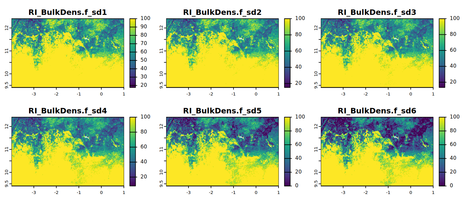
# extract third layer of all the factor from RI object
all.factors.sd <- lapply(RI, function(l) l[[3]])
all.factors.sd <- do.call(c, all.factors.sd)
# map visualization of soil property data for a specific sd
plot(all.factors.sd[[1:6]], mar=c(1, 1.5, 2, 4))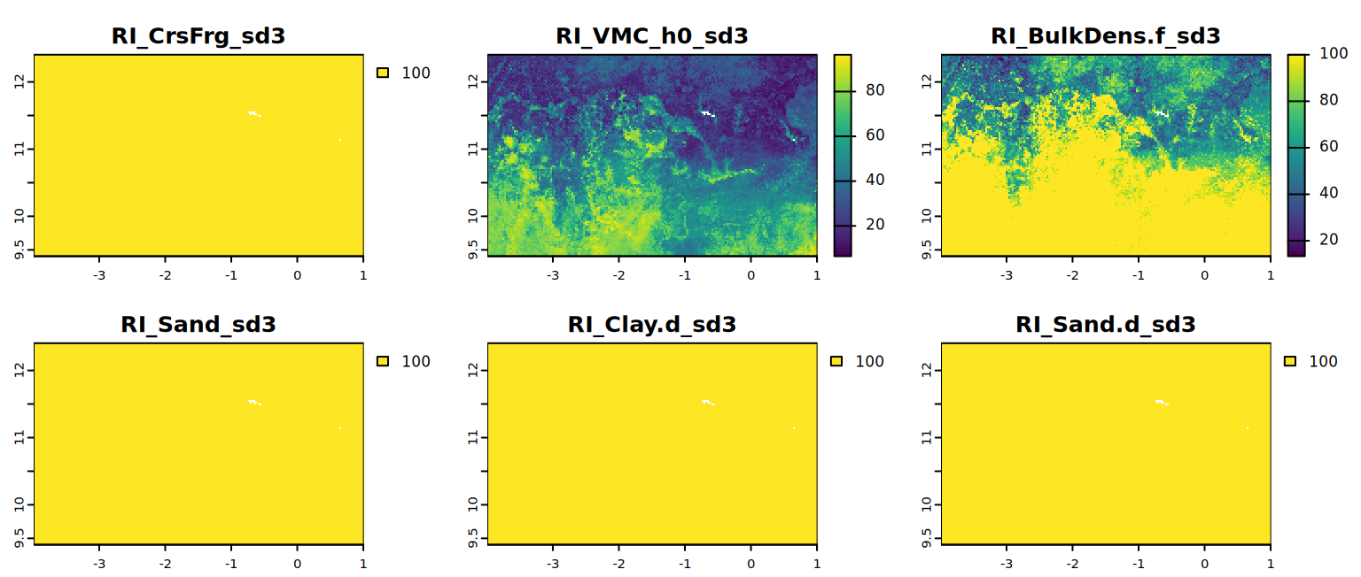
# map visualization of soil property data for a specific sd
plot(all.factors.sd[[7:12]], mar=c(1, 1.5, 2, 4))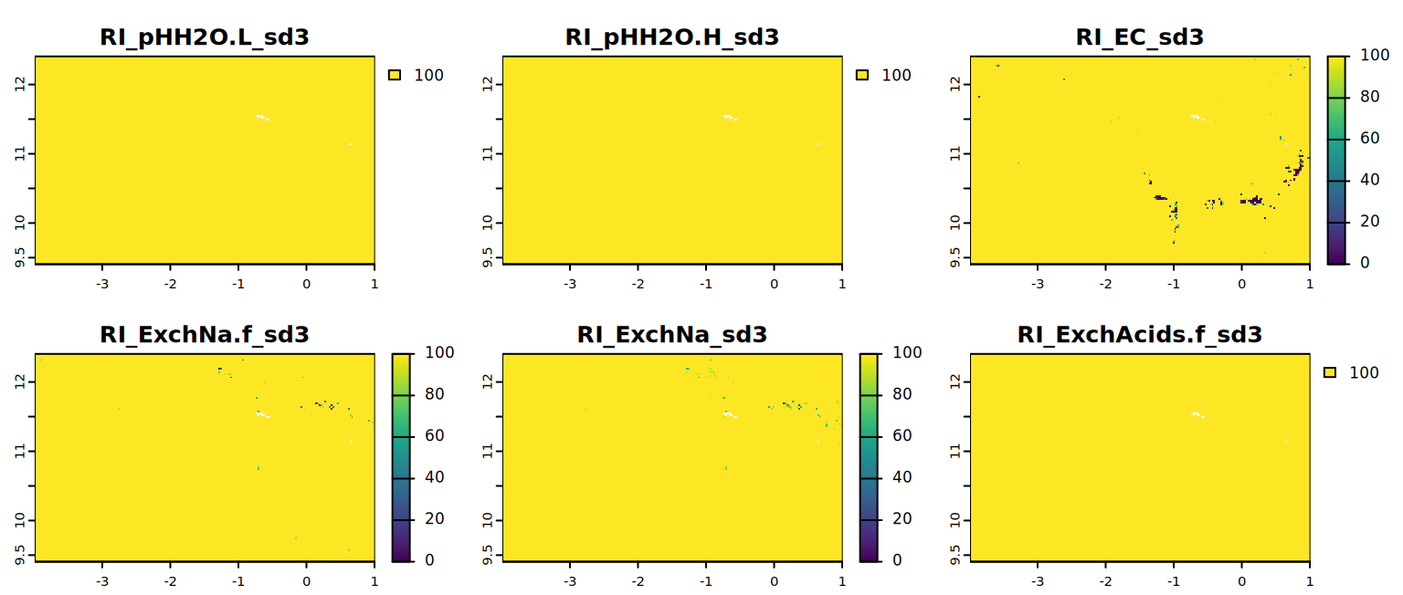
Hint: You can plot other rootability indexes by changing “BulkDens.f” with another soil factor, or another depth interval by changing [[3]] to eg [[2]].
Also we can show the statistics for the different factors per depth interval.
print(rn[2]); stats.all(RI[[1]]) # this is RI for CrsFrg
print(rn[3]); stats.all(RI[[2]])
print(rn[4]); stats.all(RI[[3]])
print(rn[5]); stats.all(RI[[4]])
print(rn[6]); stats.all(RI[[5]])
print(rn[7]); stats.all(RI[[6]])
print(rn[8]); stats.all(RI[[7]])
print(rn[9]); stats.all(RI[[8]])
print(rn[10]); stats.all(RI[[9]])
print(rn[11]); stats.all(RI[[10]])
print(rn[12]); stats.all(RI[[11]])
print(rn[13]); stats.all(RI[[12]])
print(rn[14]); stats.all(RI[[13]])
# print(rn[15]); stats.all(RI[[14]])
# print(rn[16]); stats.all(RI[[15]])
Next step is to evaluate for each factor if the rootability index is limited beyond (below) the threshold index in any of the depth intervals and assess for each factor the average depth of the depth interval where this is the case (not the upper depth of the interval). This factor-specific depth (factorDpth) is 200 cm if the index is not beyond the threshold index in any of the intervals and otherwise 2.5, 10, 22.5, 45, 80 or 150 cm.
# calculate the average depth of the depth interval
hdepth <- (UpDpth+LowDpth) / 2

# loop through factors
for(i in 2:length(rn)) {

  # apply function RI.evaluation per row of the data frame
  df <- apply(data.frame( values(RI[[i-1]] ) ), 1, FUN = RI.evaluation,
              bottom = 200, threshold.LRI = thresholds[i - 1, 4])
  # create a raster equal dimensions of the aoi and assign the results
  dummy <- create.raster(paste0(rn[i], "Dpth"), mask, as.numeric(df))
  # rename
  assign(paste0(rn[i], "Dpth"),  dummy)
}
To calculate more precise depths, we will first interpolate (using the ‘smooth.spline’ function) the rootability indices per factor from the 6 depth intervals to 200 intervals of 1 cm each and then evaluate for each factor if the rootability index is limited beyond the threshold index in any of the 200 cms. Assess for each factor the shallowest depth where this is the case. This factor-specific depth (factorDpth) is 200 cm if the index is not beyond the threshold index in any of the intervals.
hdepth <- (UpDpth+LowDpth) / 2
spline <- list(NULL)

# this step will required some time!
system.time(
  for(i in 1:15) {
    spline[[i]] <- data.frame(apply(as.data.frame(values(RI[[i]])),
                                    1, FUN = spline.apply, hdepth,
                                    interval = 200, steps = 1))
  }
)
And again we will repeat above step to calculate the factor specific depths (factorDpths_spl) but now using the result of the interpolation as input.
for(i in 2:length(rn)) {

  df <- apply(data.frame(spline[[ i - 1]]), 2, FUN = RI.evaluation,
               bottom = nrow((spline[[i - 1]])),
               threshold.LRI = thresholds[i - 1, 4])
  # create a raster equal dimensions of the aoi and assign the results
  dummy <- create.raster(paste0(rn[i], "Dpth_spl"), mask, as.numeric(df))
  assign(paste0(rn[i], "Dpth_spl"),  dummy) # rename
}
We give the statitics and maps to compare both results and select an approach.
map <- c(BulkDens.fDpth, BulkDens.fDpth_spl)
plot(map, mar = c(1, 1.5, 2, 4)) # mar = c(bottom, left, top and right)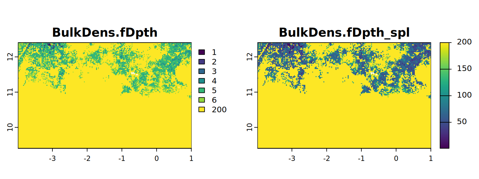
#stats.all(map)

map <- c(CrsFrgDpth, CrsFrgDpth_spl)
plot(map, mar = c(1, 1.5, 2, 4))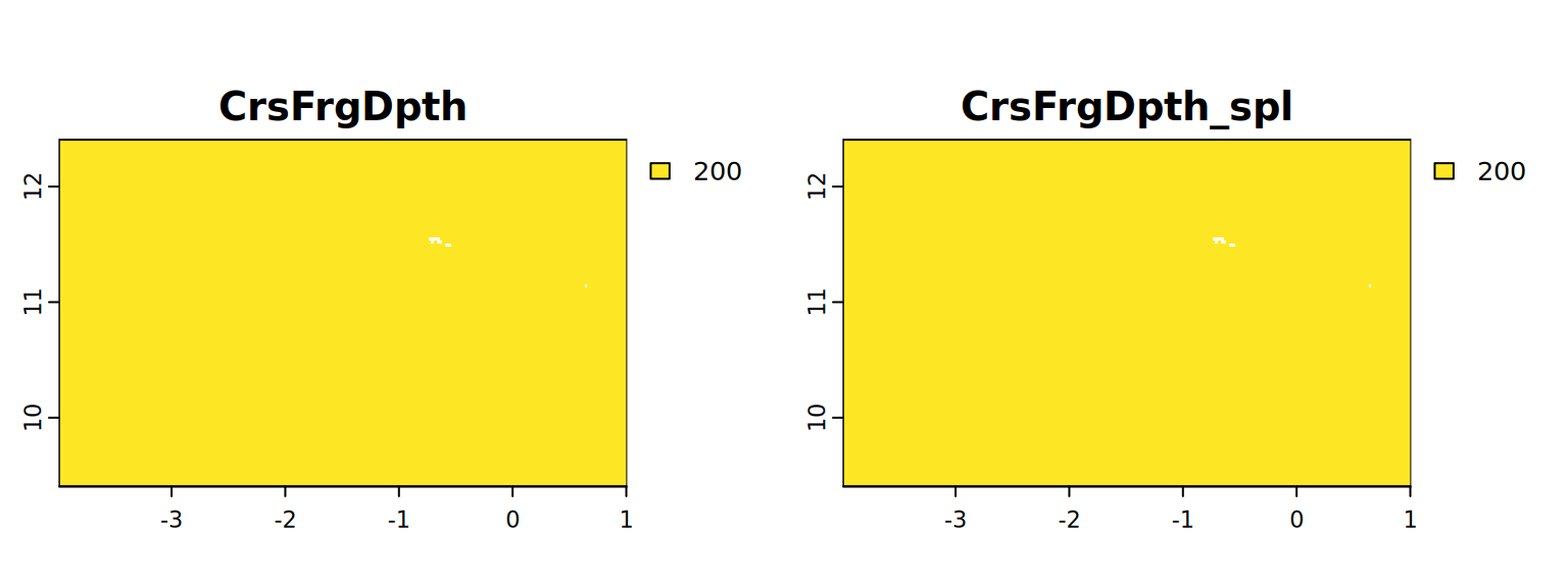
#stats.all(map)

map <- c(VMC_h0Dpth, VMC_h0Dpth_spl)
plot(map, mar = c(1, 1.5, 2, 4))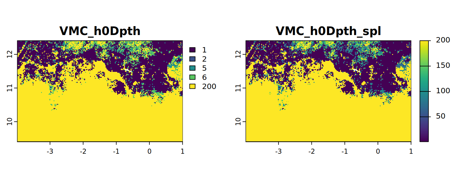
#stats.all(map)

map <- c(SandDpth, SandDpth_spl)
plot(map, mar = c(1, 1.5, 2, 4))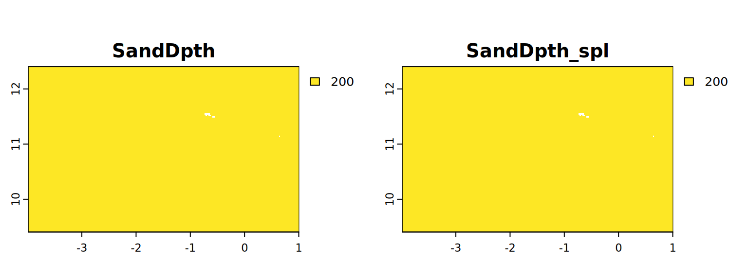
#stats.all(map)

map <- c(Clay.dDpth, Clay.dDpth_spl)
plot(map, mar = c(1, 1.5, 2, 4))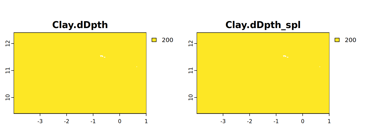
#stats.all(map)

map <- c(Sand.dDpth, Sand.dDpth_spl)
plot(map, mar = c(1, 1.5, 2, 4))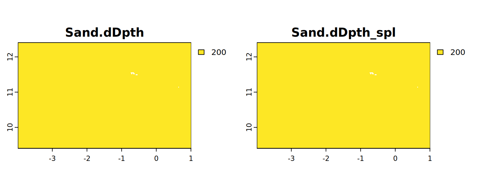
#stats.all(map)

map <- c(pHH2O.LDpth, pHH2O.LDpth_spl)
plot(map, mar = c(1, 1.5, 2, 4))
#stats.all(map)

map <- c(pHH2O.HDpth, pHH2O.HDpth_spl)
plot(map, mar = c(1, 1.5, 2, 4))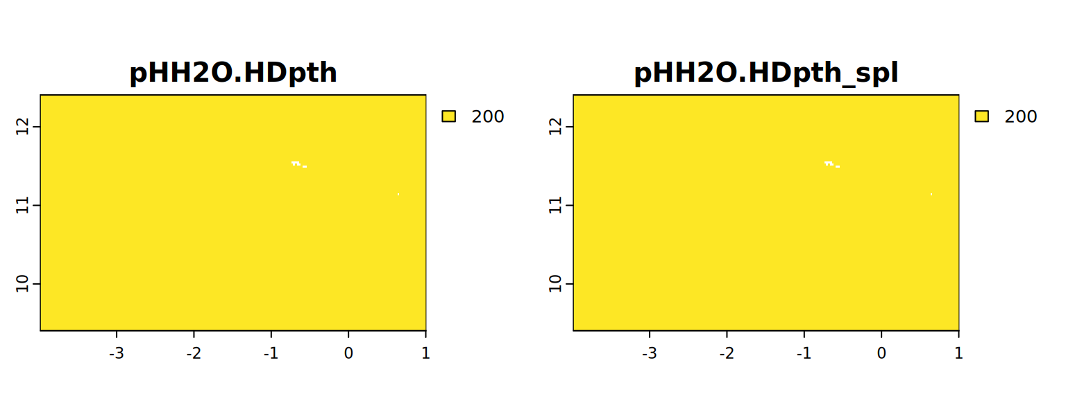
#stats.all(map)

map <- c(ECDpth, ECDpth_spl)
plot(map, mar = c(1, 1.5, 2, 4))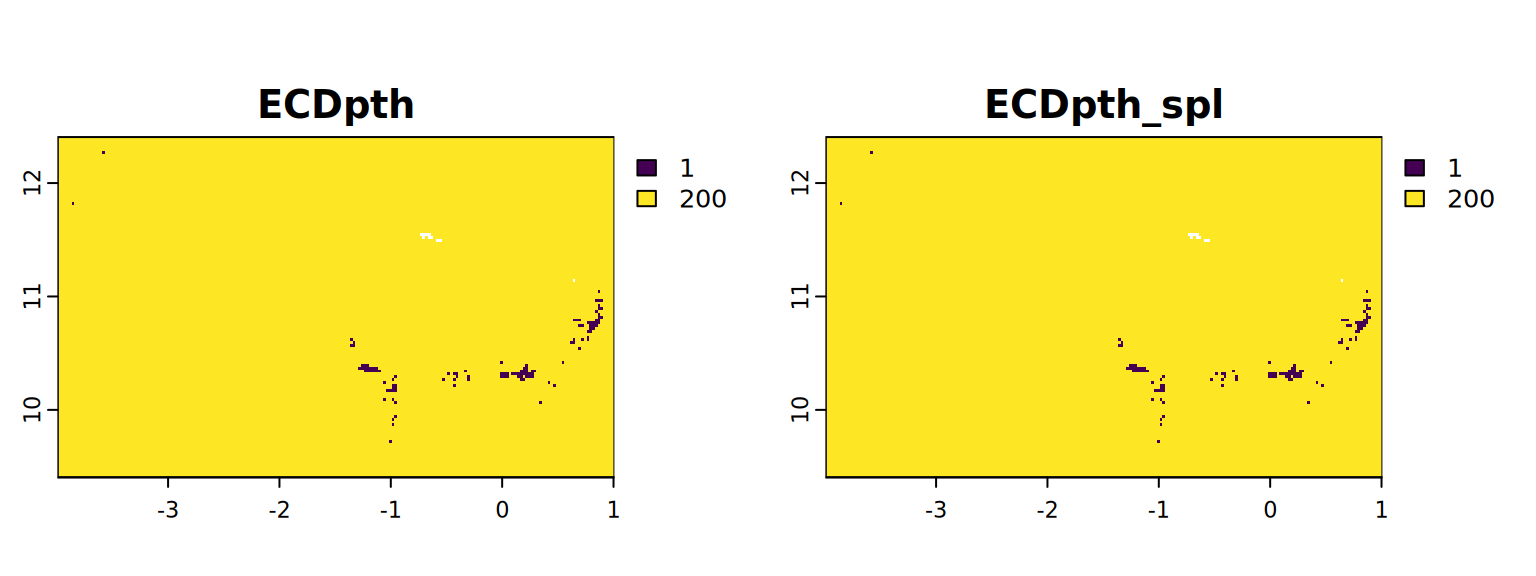
#stats.all(map)

map <- c(ExchNa.fDpth, ExchNa.fDpth_spl)
plot(map, mar = c(1, 1.5, 2, 4))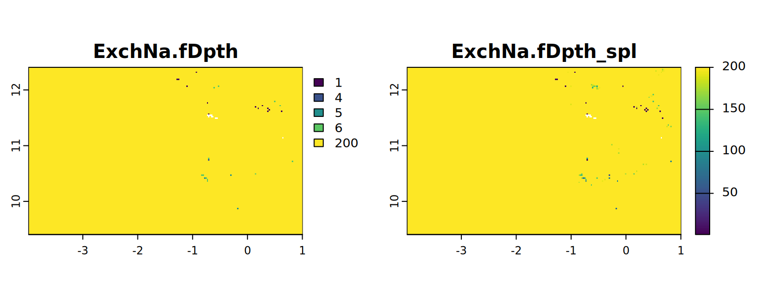
#stats.all(map)

map <- c(ExchNaDpth, ExchNaDpth_spl)
plot(map, mar = c(1, 1.5, 2, 4))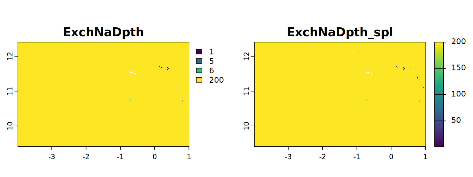
#stats.all(map)

map <- c(ExchAcids.fDpth, ExchAcids.fDpth_spl)
plot(map, mar = c(1, 1.5, 2, 4))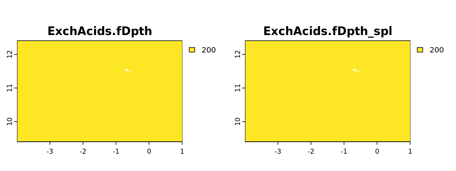
#stats.all(map)

map <- c(ExchAcidsDpth, ExchAcidsDpth_spl)
plot(map, mar = c(1, 1.5, 2, 4))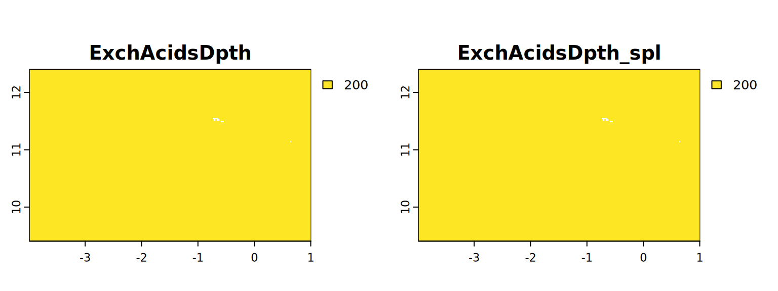
#stats.all(map)It appears with the spline approach we have more detail. So from now on we will use these results (from 4.3).
Compare the various factorDpth_spl’s (splined depths of soil where rootability is restricted beyond the threshold index for each of the factors) with the depth of soil to bedrock, the depth of soil to oxygen shortage (derived from drainage class) and the depth that maize can maximally root (150 cm). The shallowest of these depths is the soil rootable depth (RZD) in cm.
First calculate the aerated depth (depth to groundwater or depth to oxygen shortage) from drainage classes.
# depth to oxygen shortage
drainClassesLegend <- data.frame(drainClasses = c(1, 2, 3, 4, 5, 6, 7),
                                 mdepth = c(10, 40, 75, 115, 160, 210, 265))
## get effective depths per drainage class:
drainClasses.v <- data.frame(values(drainClasses))
drainDpth <- plyr::join(drainClasses.v, drainClassesLegend, type = "left",
                        match = "first")$mdepth
summary(drainDpth)
values(drainClasses) <- drainDpth
drainDpth <- drainClasses
Preparing all the depths we need in one stack.
factor_depth.ri <- lapply(paste0(rn[2:16], "Dpth_spl"), function(x) {get(x)})
factor_depth.ri <- do.call("c", factor_depth.ri)
rzd <- c(drainDpth, RockDpth, CropDpth, factor_depth.ri)
rzd <- mask(rzd, mask)
plot(drainDpth, main = "drainDpth", mar = c(1.2, 0.5, 1.5, 1))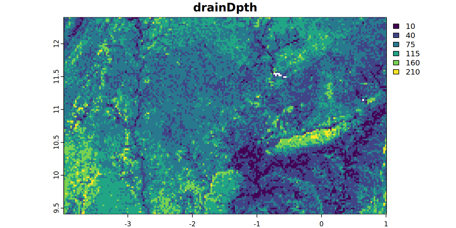
#stats(drainDpth, 1)
plot(RockDpth, main = "RockDpth", mar = c(1.2, 0.5, 1.5, 1))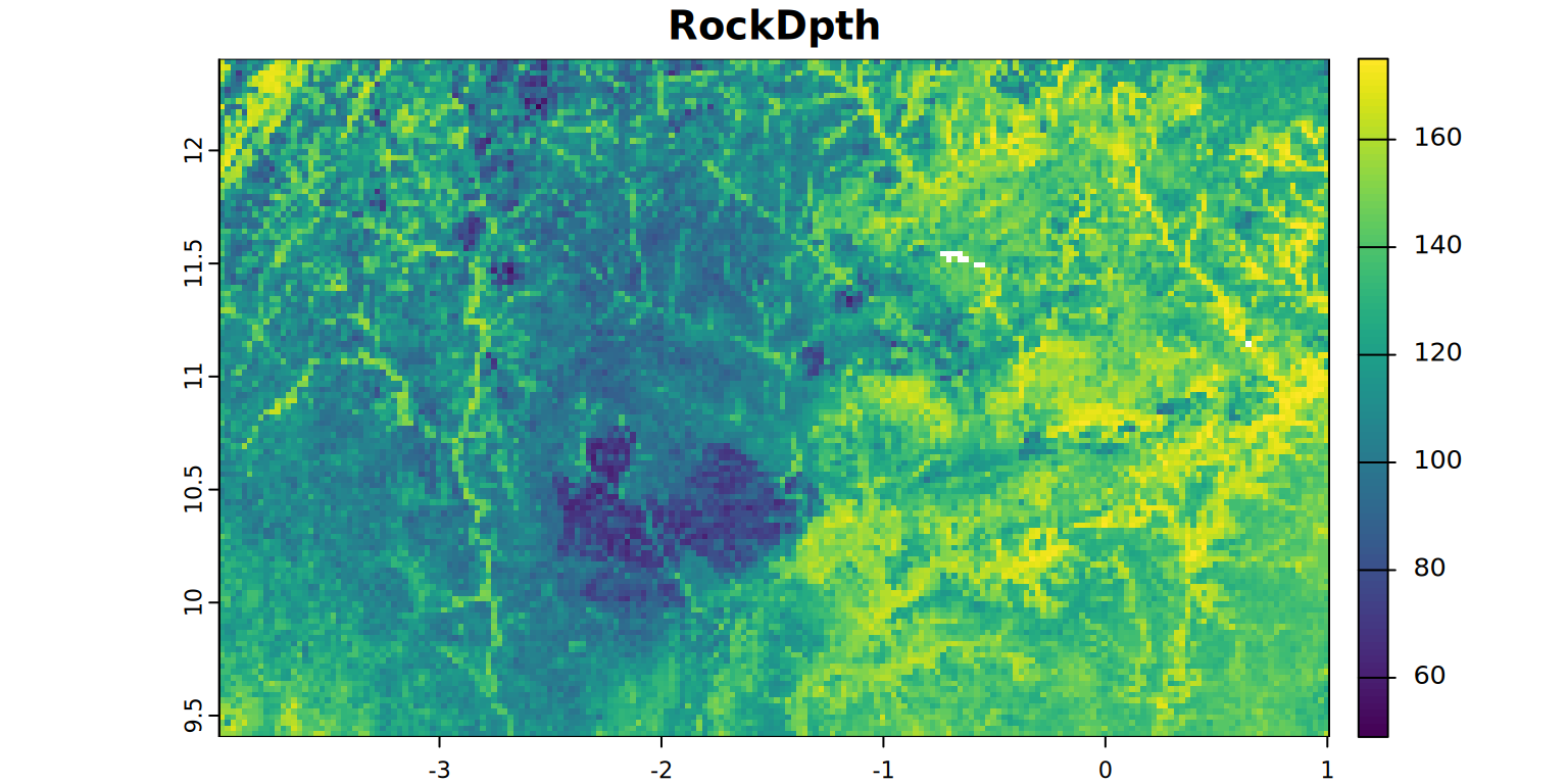
#stats(RockDpth, 1)Next step compares the factor-specific shallowest depths with each other and also with the depth to bedrock, to oxygen shortage and to the genetically defined maximum depth the selected crop (maize) can extend its rooting system to evaluate the shallowest depth at which rootability is restricted, defining the soil rootable depth or the effective root zone depth (RZD). Description: JGB Leenaars et al., 2018.
A map and the statistics of the rootable depth (cm) will be produced.
rzd.min <- app(rzd, 1, fun = min, na.rm = TRUE)
rzd.min <- mask(rzd.min, mask)
plot(rzd.min, main = "rzd.min", mar = c(1.2, 0.5, 1.5, 1))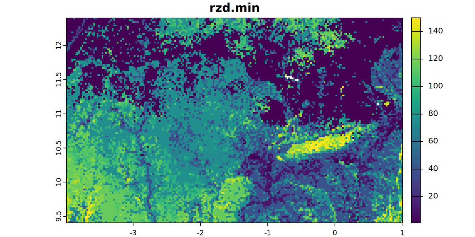
names(rzd.min) <- "rzd" # na data
#stats.all(rzd.min)
We will now identify which soil factor was the limiting rootable depth.
# this step will required some time!
limiting.factor <- apply(values(rzd), 1,
                         function(x) {
                          colnames(values(rzd))[which(x == min(x, na.rm=TRUE))[1]]
                          })

limiting.factor <- data.frame(limiting.factor,
                              as.numeric(as.factor(limiting.factor)))
rzd.r <- rzd[[1]]
names(rzd.r) <- "limitingFactor"
# check what is happening
values(rzd.r) <- limiting.factor[, 2]
plot(rzd.r, main = "rzd.r", mar = c(1.2, 0.5, 1.5, 1))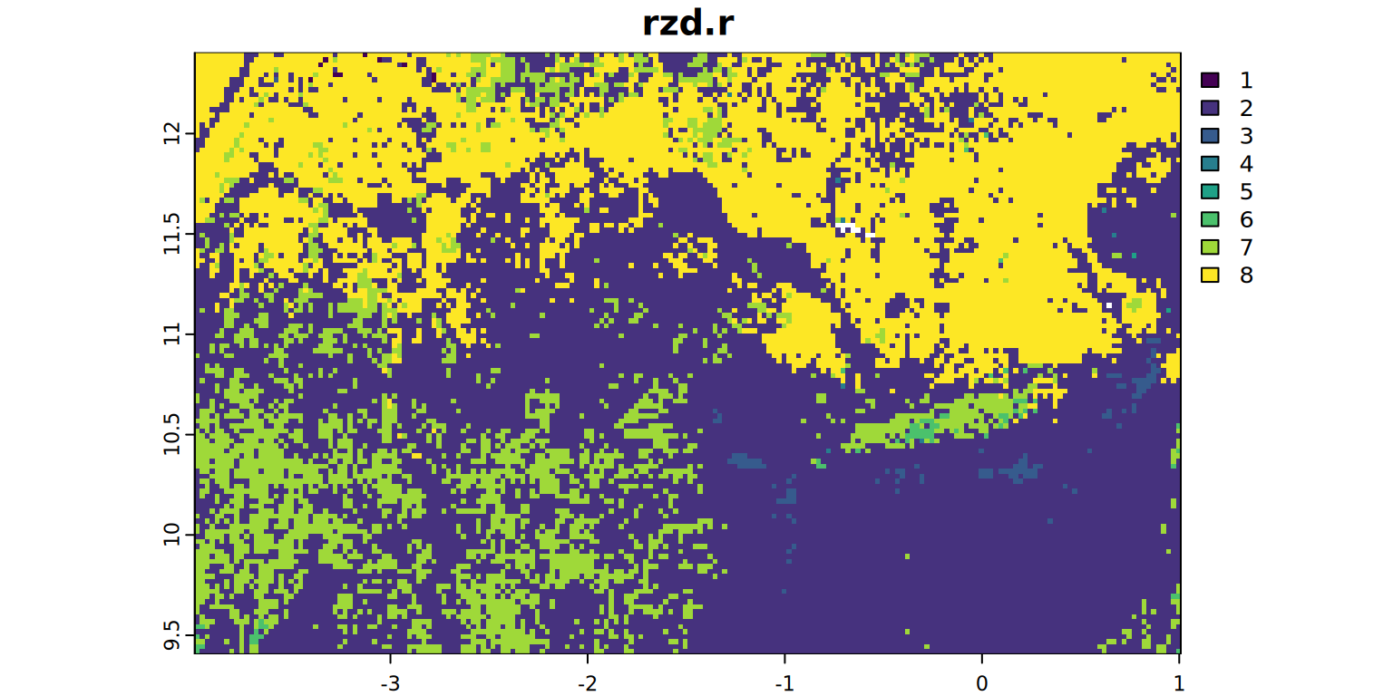
legend <- data.frame(limitingFactor = unique(limiting.factor)[[1]],
                     value = unique(limiting.factor)[[2]])
(legend <- legend[order(legend$value), ])
limitingFactor value
3 BulkDens.fDpth_spl 1
2 drainClasses 2
5 ECDpth_spl 3
6 ExchNa.fDpth_spl 4
9 ExchNaDpth_spl 5
7 pHH2O_sd1 6
4 RockDpth 7
1 VMC_h0Dpth_spl 8
8 <NA> NA(summary <- freq(rzd.r, digits = 0)) layer value count
1 1 1 10
2 1 2 13704
3 1 3 118
4 1 4 9
5 1 5 2
6 1 6 69
7 1 7 3228
8 1 8 6850Now we’ll calculate the impact of the rootable depth on the Root Zone Plant-Available Water Holding Capacity (RZ-PAWHC in mm) from the weighted sum of Effective PAWHC_mm’s (mm) of the depth intervals within the RZD.
- UpDpth <- c(0,5,15,30,60,100)
- LowDpth <- c(5,15,30,60,100,200)
A map and the statistics of the RZ-PAWHC (mm) will be produced.
r <- c(EffPAWHC_mm, rzd.min)

weighted_sum <- apply(values(r), 1, function(x) {

  if (all(!is.na(x))){

    rzd <- x["rzd"]

    df <- data.frame(upDpth = c(0, 5, 15, 30, 60, 100),
                    lowDpth = c(5, 15, 30, 60, 100, 200))

    # redefining the ranges of the upper and lower depths of each depth interval
    # is this necessary?
    df$minDpth <- ifelse(df$upDpth <= 0, yes = 0, no = df$upDpth)
    df$minDpth <- ifelse(df$upDpth >= rzd, yes = rzd, no = df$minDpth)
    df$maxDpth <- ifelse(df$lowDpth >= rzd, yes = rzd, no = df$lowDpth)

    # determine the thickness of each individual depth interval
    # (lowDpth-upDpth) of each profile
    df$depth <- df$maxDpth - df$minDpth
    df$depth.interval <- df$lowDpth - df$upDpth

    wt <- df$depth / df$depth.interval # do you also call this factor?

    weighted_sum <- sum(x[1:length(x) - 1] * wt)

  } else {

    weighted_sum <- NA

  }
})

RZPAWHC <- create.raster("RZPAWHC", mask, weighted_sum)
#stats.all(RZPAWHC)
#stats.all(EffTPAWHC_mm)
plot(c(RZPAWHC, EffTPAWHC_mm), mar = c(1, 1.5, 2, 4))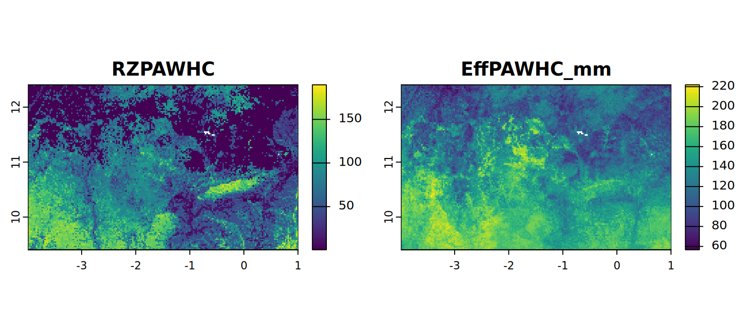
RZ-PAWHC is needed for the next section. Here we show how to export an output using the writeRaster() function from terra. Nevertheless, the RZPAWHC.tif is available to the user in the “nutrients” folder. The overwrite, filetype and datatype arguments are optional. Check the writeRaster() documentation here: rdrr.io/cran/terra/writeRaster for more information about the arguments.
saving_path <- file.path(workingDir, "output/RZPAWHC.tif")
writeRaster(RZPAWHC, filename = saving_path,
            overwrite = TRUE, filetype = "COG", datatype = "FLT4S")

## end of script