# Empty memory and workspace
gc()
rm(list = ls())

# Modify this file path with the location where you saved the tutorial files
workingDir <- file.path("C:/soil_water_nutrients")

# Set up working directories
setwd(workingDir)
scripts_path <- file.path(workingDir, "code/functions")
filesDir <- file.path(workingDir, "nutrients")3 Mapping nutrients
3.1 Practical soil nutrient availability
Required libraries and external functions for this section:
# Load libraries
require(terra)
require(knitr)

# Call external functions
source(file.path(scripts_path, "Auxiliary_functions.R"))
Soil nutrient availabilities are calculated from the available data on soil nutrient contents. The data on soil nutrient contents are aggregated for the topsoil of 0-30 cm from data provided by the Africa SoilGrids for standard depth intervals 0-5 cm, 5-15 cm and 15-30 cm. (These Africa SoilGrids are the result from spatial predictions based on original lab data measured from georeferenced soil samples).
The nature of the lab methods used defines the nature of the soil nutrient contents measured and mapped (e.g. extractable P content by Mehlich3 is not similar to extractable P content by Olsen nor the Total P content or the plant-available P content in solution). The availability of the nutrients, dissolved in the soil solution and available for crop uptake, is only a fraction of the measured and mapped content of the nutrients and is estimated for N, P and K using the PTFs in QUEFTS. QUEFTS is a model for QUantitative Evaluation of the Fertility of Tropical Soils developed by Janssen et al. (1990) and updated by Sattari et al. (2014). The PTF’s are used here as an internal function called ‘QUEFTS soil nutrient ávailability’
The soil properties used as variables in QUEFTS are pHH2O, TotalN, OrgC, ExtrP_olsen, TotalP, ExchK and Temprtr. The corresponding soil property data available from the Africa SoilGrids are pHH2O, TotalN, OrgC, ExtrP, TotalP, ExtrK and Temprtr. Note though that the definition of some of these properties do not match 1 to 1 and few data conversions are necessary (e.g. ExtrP (mehlich 3) to ExtrP_olsen and ExtrK (mehlich 3) to ExchK_nh4ac whereby also some of the units need to be converted) which we’ll do here.
Africa soilgrids data available and required as input data for the (internal) function ‘quefts soil nutrient availability’ and already converted (1 value for the topsoil (0-30 cm) per pixel):
- CrsFrg = volumetric coarse fragments content (m3/100m3) (0-30 cm)
- BulkDens = bulk density of the fine earth fraction * 1000 (kg/m3) (0-30 cm) -> divide by 1000
- pHH2O = pHH2O (0-30 cm) * 10 / 10 -> already divided by 10
- OrgC = organic C content (g/kg) (0-30 cm)
- TotalN = total N content (mg/kg) (0-30 cm) -> divide by 1000
- TotalP = total P content (mg/kg) (0-30 cm)
- ExtrP = mehlich3 extractable P content (mg/100kg) (0-30 cm) -> divide by 100 and convert to P_olsen
- ExtrK = mehlich3 extractable K content (mg/kg) (0-30 cm) -> convert to mmolc/kg and to Exchangeable K
- Temprtr = soil temperature avg from day and night (deg celcius) (0-30 cm)
Read the Africa SoilGrids data.
TotalN <- rast(file.path(filesDir, "TotalN_0_30cm.tif")) # g/kg
TotalP <- rast(file.path(filesDir, "TotalP_0_30cm.tif")) # mg/kg
Temprtr <- rast(file.path(filesDir, "Temprtr.tif")) # C
pHH2O <- rast(file.path(filesDir, "pHH2O_0_30cm.tif")) # * 1
OrgC <- rast(file.path(filesDir, "OrgC_0_30cm.tif")) # g/kg
BulkDens <- rast(file.path(filesDir, "BulkDens_0_30cm.tif")) # kg/dm3
ExtrK <- rast(file.path(filesDir, "ExtrK_0_30cm.tif")) # mg/kg
ExtrP <- rast(file.path(filesDir, "ExtrP_0_30cm.tif")) # mg/100kg
CrsFrg <- rast(file.path(filesDir, "CrsFrg_0_30cm.tif")) # m3/100m3
Convert the Africa SoilGrids data to the properties and units required as input for the (internal) function ‘QUEFTS soil nutrient availability’. Exchangeable K (by NH4OAc in mmolc/kg) is derived from extractabkle K (by Mehlich3 in mg/kg) and extractable P by Olsen from extractable P by Mehlich 3.
## Units conversions with above indications
TotalN <- TotalN / 1000 # total N, in ppm. Convert ppm to g/kg (divide by 1000)
BulkDens <- BulkDens / 1000 # convert BulkDens in kg/m3 to kg/dm3 (divide by 1000)
ExchK <- 0.03 * ExtrK #  K-m3 in ppm, ExchK in mmolc/kg and measured in NH4.

# Polsen in ppm calculate from P-m3 in pp100m
Polsen <- lapp(c(pHH2O, ExtrP), fun = function(pHH2O, ExtrP) {

  ifelse(pHH2O < 6.5, 0.55 * (ExtrP/100),
         ifelse(pHH2O < 7.3, 0.5 * ExtrP/100, 0.45 * ExtrP/100))
})
summary(TotalN)
summary(ExtrP)
summary(Polsen)
summary(ExtrK)
summary(ExchK)
summary(BulkDens)

# Properties where no conversions needed
summary(pHH2O)
summary(OrgC)# OrgC in g/kg,  no conversion needed
summary(TotalP)# TotalP no conversion needed
summary(CrsFrg)# CrsFrg  no conversion needed
summary(Temprtr)# annual mean temperature
The input data on soil nutrient contents are expressed as relative contents (e.g. mg/kg) and we like to have an idea about the absolute contents or quantity (kg/ha in 0-30 cm depth = kg/3000 m3). This conversion requires input data on bulk density. We’ll calculate effective quantities by also considering the volumetric coarse fragments content (that volume of soil doesn’t contain soil nutrients).
# Effective quantity in 0-30 cm soil (kg/ha.30 cm)
# (kg organic C/ha) #3000 = 0.3m * 10000m2)
C_effqnt <- OrgC * BulkDens * (100 - CrsFrg)/100 * 3000
# (kg total N/ha)
N_effqnt <- round(TotalN * BulkDens * (100 - CrsFrg)/100 * 3000, 1)
#(kg total P/ha)
Pt_effqnt <- TotalP * BulkDens * (100 - CrsFrg)/100 * 3000/1000
#(kg P olsen/ha)
P_effqnt <- round(Polsen * BulkDens * (100 - CrsFrg)/100 * 3000/1000, 1)
# (kg exchangeable K/ha) # 39 to convert from mmol to kg
K_effqnt <- round(ExchK * 39 * BulkDens * (100 - CrsFrg)/100 * 3000/1000, 1)
Now produce the statistics and maps of the absolute soil nutrient contents.
# Effective quantity in 0-30 cm soil (kg/ha.30 cm)
effqnt <- c(C_effqnt, N_effqnt, Pt_effqnt, P_effqnt, K_effqnt)
names(effqnt) <- c("C_effqnt", "N_effqnt", "Pt_effqnt", "P_effqnt", "K_effqnt")
plot(effqnt, mar = c(1, 1.5, 2, 4)) # mar = c(bottom, left, top and right)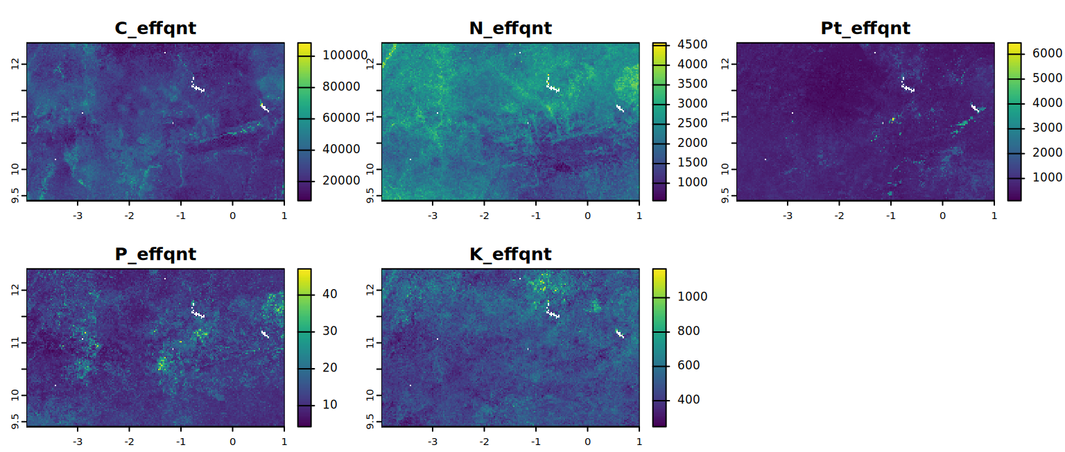
summary <- stats.all(effqnt)
kable(summary)
Next step is to calculate the effective availability or supply of N, P and K (kg/ha). The availability of N, P and K, as a fraction of the measured and mapped contents of N, P and K, is calculated using the formulas proposed by Satarri et al. (2014). These calculations are done from the relative contents, rather than the absolute contents that we just calculated, of N, P and K in the topsoil (TotalN, ExtrP_olsen and ExchK) as well as from other soil properties of the topsoil (OrgC, TotalP, pHH2O and soil temperature - Temprtr). From these maximal availabilities we’ll calculate the effective availabilities by deducting the volumetric fraction of coarse fragments and by assuming that only 85% of the availability is indeed available for crop uptake. The availabilities are a function of pH and first we’ll calculate these correction factors for pH.
# Effective nutrient availability (supply) from 0-30 cm soil (kg/ha.30 cm)

# Correction factor for pH-H2O (see Sattari)

ExtrP_olsen <- lapp(c(pHH2O, ExtrP), fun = function(pHH2O, ExtrP) {
  ifelse(pHH2O < 6.5, 0.55 * (ExtrP / 100),
         ifelse(pHH2O < 7.3, 0.5 * ExtrP / 100,
                0.45 * ExtrP / 100))
} )

pHfN <- app(c(pHH2O), fun = function(pHH2O) {
  # for nitrogen (from Sattari)
  ifelse(pHH2O < 4.7, 0.4, ifelse(pHH2O >= 7, 1, 0.25 * (pHH2O - 3)))
})

pHfP <- app(c(pHH2O), fun = function(pHH2O) {
  # phosphorus (Sattari)
  ifelse(pHH2O < 4.7, 0.02,
         ifelse(pHH2O < 6, 1 - 0.5 * (pHH2O - 6)^2,
                ifelse(pHH2O<6.7, 1,
                       ifelse(pHH2O < 8, 1 - 0.25 * (pHH2O - 6.7)^2, 0.57))))})


pHfK <- app(pHH2O, fun = function(pHH2O) {
  # Potassium; (from Sattari)
  ifelse(pHH2O < 4.5, 1, ifelse(pHH2O  >= 6.8, 0.6, 6.1 * pHH2O^(-1.2)))
})


# Potential nutrient availability (supply) from 0-30 cm soil (kg/ha.30 cm)
sn_oc <- lapp(c(pHfN, Temprtr, OrgC),
             fun = function(pHfN,Temprtr,OrgC) {
               pmax(pHfN * 2 * 2^((Temprtr-9)/9) * OrgC, 0)})

sn_tn <- lapp(c(pHfN,Temprtr, TotalN),
             fun = function(pHfN,Temprtr,TotalN) {
               pmax(pHfN * 20*2^((Temprtr-9)/9) * TotalN, 0)})

sNmx <- (sn_oc + sn_tn)/2   # mean of the two

sPmx <- lapp(c(pHfP, TotalP, ExtrP_olsen),
            fun = function(pHfP, TotalP, ExtrP_olsen) {
              pmax((pHfP * 0.014 * TotalP + 0.5 * ExtrP_olsen), 0)})

sKmx <- lapp(c(pHfK, ExchK, OrgC),
            fun=function(pHfK,ExchK,OrgC) {
              pmax((pHfK * 500 * ExchK)/(2 + 0.9 * OrgC), 0)})

c(sNmx, sPmx, sKmx)

# Effective soil nutrient supply available for uptake (considering coarse
# fragments and assuming that 85% of the supply is available for uptake)
sSUE <- 0.85 # soil supply uptake efficiency (not quefts)
sNS <- round(sSUE * sNmx * ((100 - CrsFrg)/100), 1)
sPS <- round(sSUE * sPmx * ((100 - CrsFrg)/100), 1)
sKS <- round(sSUE * sKmx * ((100 - CrsFrg)/100), 1)

c(sNS, sPS, sKS)- sNS = soil N supply effectively available for uptake (kg/ha)
- sPS = soil P supply effectively available for uptake (kg/ha)
- sKS = soil K supply effectively available for uptake (kg/ha)
Produce statistics and maps of the effective soil nutrient availability.
# Maximum availability (supply) in 0-30 cm soil (kg/ha.30 cm)
sNPKSmx <- c(sNmx, sPmx, sKmx)
names(sNPKSmx) <- c("sNmx", "sPmx", "sKmx")
plot(sNPKSmx,  mar = c(1, 1.5, 2, 4))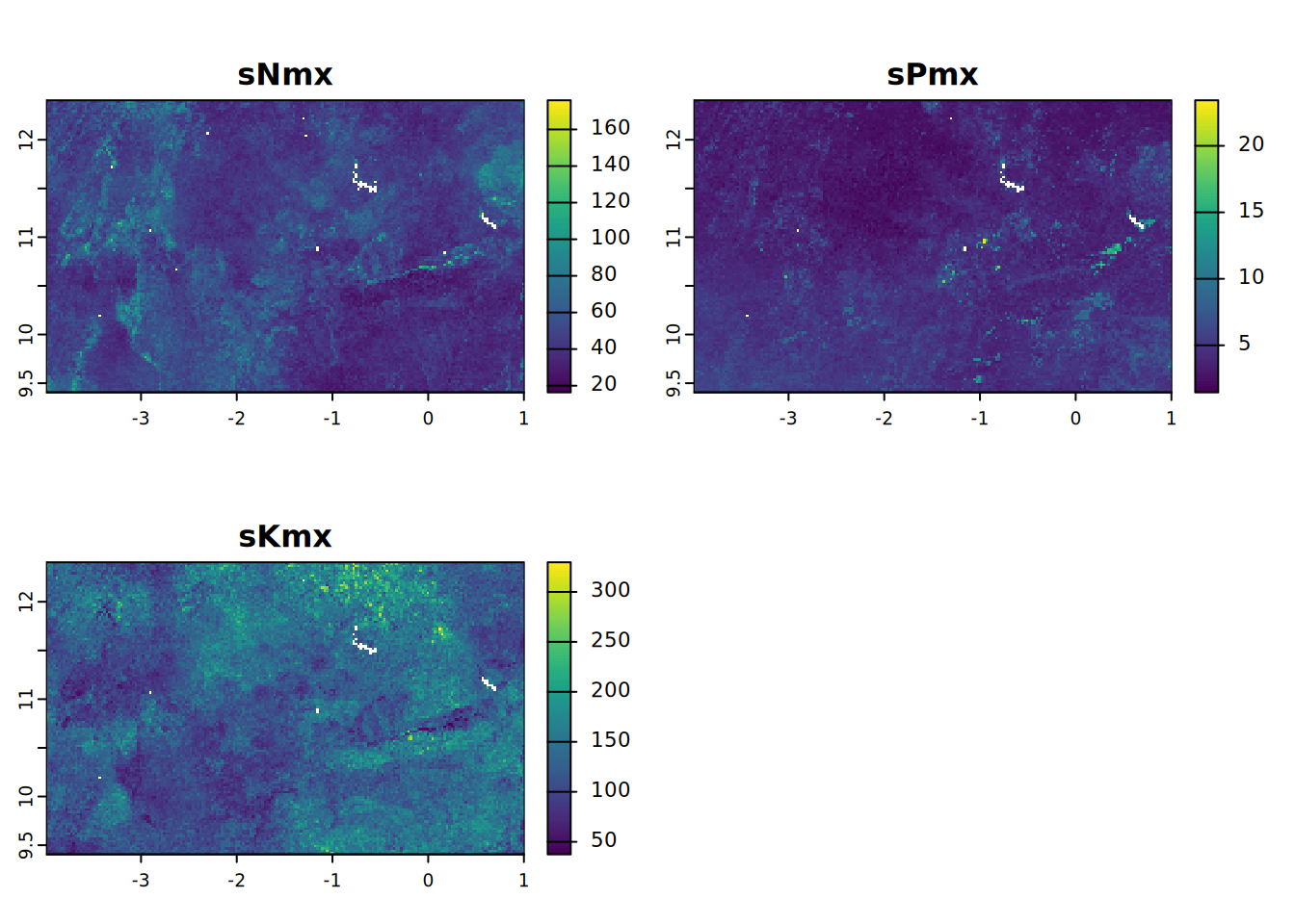
summary <- stats.all(sNPKSmx)
kable(summary)
# Effective availability (supply) in 0-30 cm soil (kg/ha.30 cm)
sNPKS <- c(sNS, sPS, sKS)
names(sNPKS) <- c("sNS", "sPS", "sKS")
plot(sNPKS, mar = c(1, 1.5, 2, 4))
summary <- stats.all(sNPKS)
kable(summary)
3.2 Practical nutrient gaps from root zone water-limited crop nutrient demand and soil nutrient supply
Water-limited crop growth and yield potentials are codetermined by the root zone plant-available water holding capacity of the soil (thus by rootable depth, coarse fragments content in the rootable depth and the plant-available water holding capacity of the fine earth fraction in the rootable depth). Crop growth simulation models like e.g. WOFOST, DSSAT, LINTUL, APSIM and others do require these soil data as model input. We’ll not calculate water-limited yield using such model here but instead refer to water-limited yield potentials read from existing maps produced using similar models.
The Global Yield Gap Atlas (GYGA) portal provides access to data and global maps of, a. o., water-limited yield potentials for a range of crops. Also the Global Agro-Ecological Zoning (GAEZ) portal of IIASA/FAO provides access to data and global maps of, a. o., yield potentials for a range of crops. The maps of GAEZ reflect attainable yield potentials which are derived from water-limited yield potentials and limited by 1) water availability assuming a rootable depth of 100 cm, 2) P&D prevalence and 3) management regime. Used as an example in this tutorial is a GAEZ map of the maize yield that is maximally attainable with an intermediate management regime (ymax).
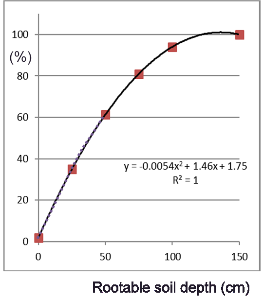
The attainable yield (ymax) is thus limited by water availability assuming a soil rootable depth of 100 cm. This yield is likely not attainable on shallower soils where water availability is lower and RZD should had been included as a variable in the original crop growth simulations. Instead, we estimate the attainable root zone water-limited yield (ymaxRZD) from the attainable Water-limited yield (ymax) and RZ-PAWHC using a simple rule suggested by GYGA Guilpart et al., 2017 and shown in next Figure.
To shorten the tutorial we’ll apply this rule in a later instance. First we assess the crop nutrient uptake that is required to indeed attain the attainable yield potential.
We calculate crop nutrient uptake requirements using the QUEFTS approach (QUantitative Evaluation of the Fertility of Tropical Soils) suggested by Janssen et al. (1990) and updated by Sattari et al. (2014). Herein we defined average yield/uptake efficiencies for maize in the region of approx. 47, 365, 57 kg/kg (for N, P and K), respectively. With these efficiencies, and to shorten the tutorial, we have already produced maps of nutrient uptake requirements corresponding with the target yields that we derived from the above GAEZ map of attainable water-limited yield (yMax). (Target yields were set at 0.55 of yMax). From these maps, and using above referred to rule, we’ll calculate the root zone limited crop nutrient uptake requirements for attaining root zone limited target yields.
Spatial grid data available and required as input data to the (internal) function ‘crop nutrient demand’: (1 value per pixel)
- yMaxMaize = attainable, water-limited, yield (kg/ha)
- yTargetMaize = target yield (0.55 of yMax)
- NuptReqMaize = Nitrogen uptake requirement of maize at target yield (kg/ha)
- PuptReqMaize = Phosphorus uptake requirement of maize at target yield (kg/ha)
- KuptReqMaize = Potassium uptake requirement of maize at target yield (kg/ha)
Read input maps for assessing root zone limited crop nutrient requirements which will be used at the end of the practical to assess nutrient gaps.
ymaxMaize <- rast(file.path(filesDir,  "ymaxMaize.tif"))
plot(ymaxMaize, main = "ymaxMaize", mar = c(1.2, 0.5, 1.5, 1))
# mar = c(bottom, left, top and right)stats.all(ymaxMaize)yTargetMaize <- ymaxMaize * 0.55
plot(yTargetMaize, main = "yTargetMaize", mar = c(1.2, 0.5, 1.5, 1))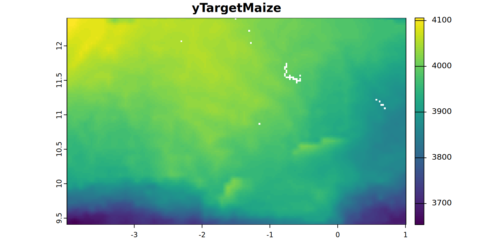
stats.all(yTargetMaize)NuptReqMaize <- rast(file.path(filesDir, "NuptReqMaize.tif"))
PuptReqMaize <- rast(file.path(filesDir, "PuptReqMaize.tif"))
KuptReqMaize <- rast(file.path(filesDir, "KuptReqMaize.tif"))
NPKuptReq <- c(NuptReqMaize, PuptReqMaize, KuptReqMaize)
plot(NPKuptReq, mar = c(1, 1.5, 2, 4))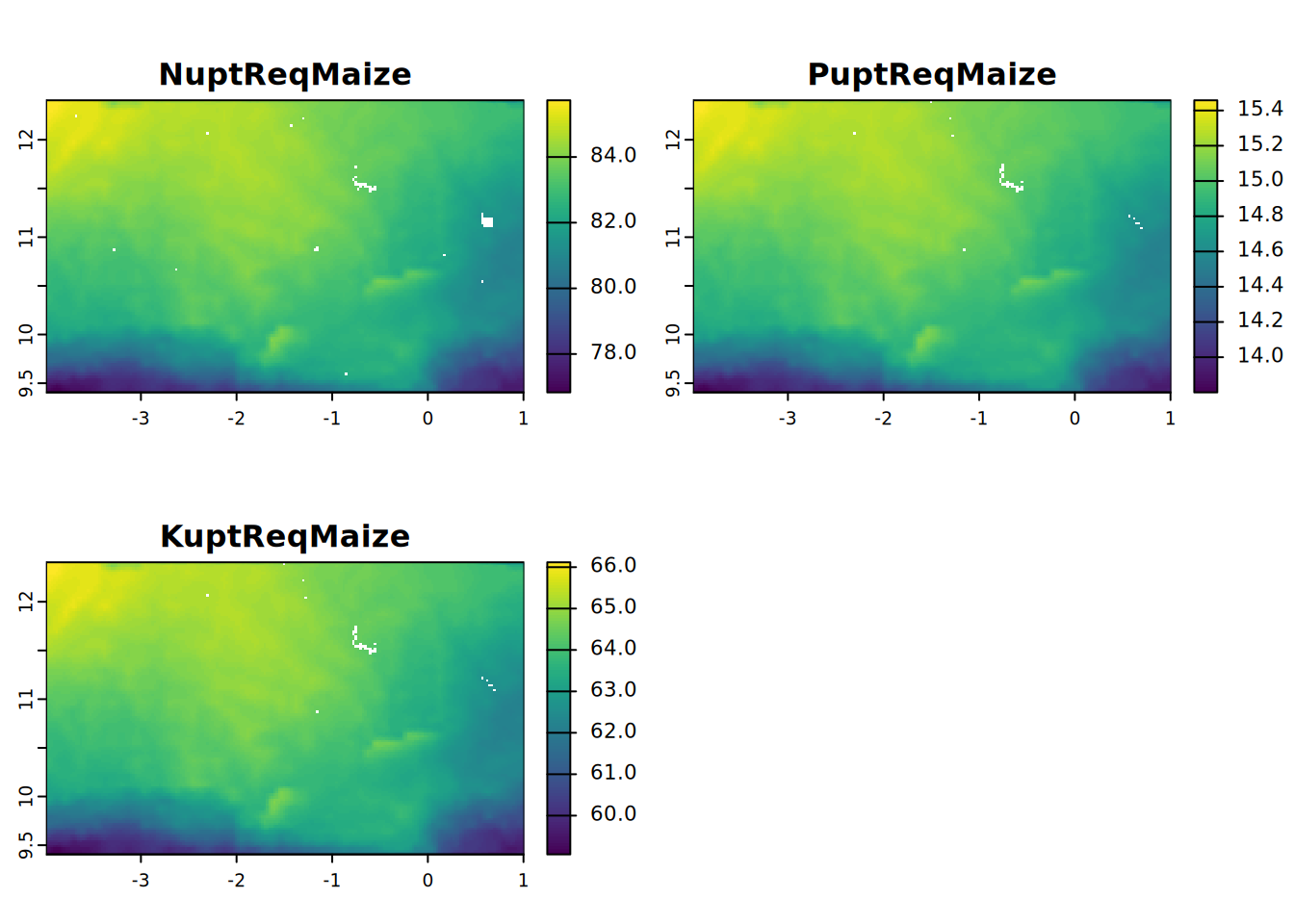
1 RzlNuptReqMaize = N uptake requirement of maize at attainable, root zone water-limited, target yield (kg/ha)
2 RzlPuptReqMaize = P uptake requirement of maize at attainable, root zone water-limited, target yield (kg/ha)
3 RzlKuptReqMaize = K uptake requirement of maize at attainable, root zone water-limited, target yield (kg/ha)
summary <- stats.all(NPKuptReq)
kable(summary)
Now we calculate the root zone limited crop nutrient uptake requirements.
# read RZPAWHC resulting from the previous section
x <- rast(file.path(filesDir, "RZPAWHC.tif"))

rzlyTargetMaize <- round(yTargetMaize * ((-0.0054*(x^2)) + (1.46*x)+(1.75))/100, 0)
names(rzlyTargetMaize) <- "rzlyTargetMaize"
(rzlyTargetMaize)
stats.all(rzlyTargetMaize)

rzlNuptReqMaize <- round(NuptReqMaize * ((-0.0054*(x^2)) + (1.46*x)+(1.75))/100, 0)
names(rzlNuptReqMaize) <- "rzlNuptReqMaize"

rzlPuptReqMaize <- round(PuptReqMaize * ((-0.0054*(x^2)) + (1.46*x)+(1.75))/100, 0)
names(rzlPuptReqMaize) <- "rzlPuptReqMaize"

rzlKuptReqMaize <- round(KuptReqMaize * ((-0.0054*(x^2)) + (1.46*x)+(1.75))/100, 0)
names(rzlKuptReqMaize) <- "rzlKuptReqMaize"

rzlNPKuptReqMaize <- c(rzlNuptReqMaize, rzlPuptReqMaize, rzlKuptReqMaize)plot(rzlNPKuptReqMaize, mar = c(1, 1.5, 2, 4))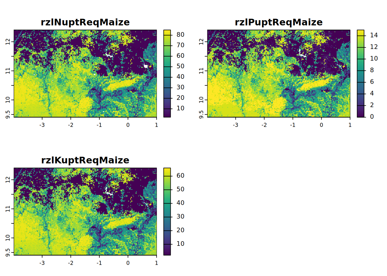
summary <- stats.all(rzlNPKuptReqMaize)
kable(summary)
3.3 Calculate nutrient gap
We calculated the crop demand for nutrients (at target yield levels) and the soil supply of nutrients. Now we’ll calculate the nutrient gap. This nutrient gap is the soil nutrient deficiency. This deficiency can be bridged by fertilisation to attain target yield. Note that we assess deficiencies relative to a spatially variable threshold rather than a spatially uniform threshold.
- Ntargetgap = N gap between supply and demand (kg/ha)
- ptargetgap = P gap between supply and demand (kg/ha)
- Ktargetgap = K gap between supply and demand (kg/ha)
Ntargetgap <- rzlNuptReqMaize - sNS #kg/ha (= fNuReq)
Ptargetgap <- rzlPuptReqMaize - sPS
Ktargetgap <- rzlKuptReqMaize - sKS
Produce statistics and maps of the nutrient gaps.
# Nutrient gaps
NPKtargetgap <- c(Ntargetgap,  Ptargetgap, Ktargetgap)
names(NPKtargetgap) <- c("Ntargetgap",  "Ptargetgap", "Ktargetgap")
plot(NPKtargetgap, mar = c(1, 1.5, 2, 4))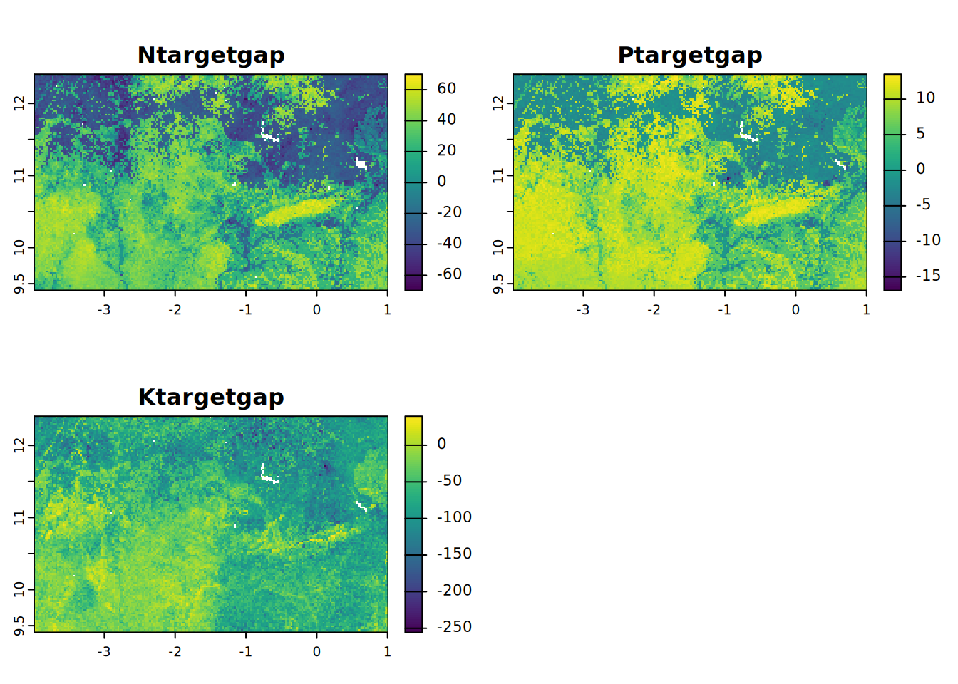
summary <- stats.all(NPKtargetgap)
kable(summary)
3.4 Calculate fertiliser nutrient recommendations
Estimate fertiliser recommendations (rates in kg/ha), assuming fixed fertiliser NPK recovery fractions (fertiliser uptake efficiencies in kg/kg). These fractions are defined from regional data as 0.4, 0.15 and 0.35 for N, P and K, respectively.
- fNR = fertiliser N recommendation (kg/ha)
- fPR = fertiliser P recommendation (kg/ha)
- fKR = fertiliser K recommendation (kg/ha)
#### if NPKtargetgap is negative then 0
Ntargetgap <- ifel(Ntargetgap < 0, 0, Ntargetgap)
Ptargetgap <- ifel(Ptargetgap < 0, 0, Ptargetgap)
Ktargetgap <- ifel(Ktargetgap < 0, 0, Ktargetgap)

# rf is simplified fertiliser recovery fraction (kg/kg)
rfN <- 0.4
rfP <- 0.15
rfK <- 0.35
fNR <- round(Ntargetgap / rfN, 0)
fPR <- round(Ptargetgap / rfP, 0)
fKR <- round(Ktargetgap / rfK, 0)
Produce statistics and maps of the fertiliser nutrient recommendations.
fNPKR <- c(fNR,  fPR, fKR)
names(fNPKR) <- c("fNR",  "fPR", "fKR")
plot(fNPKR, mar = c(1, 1.5, 2, 4))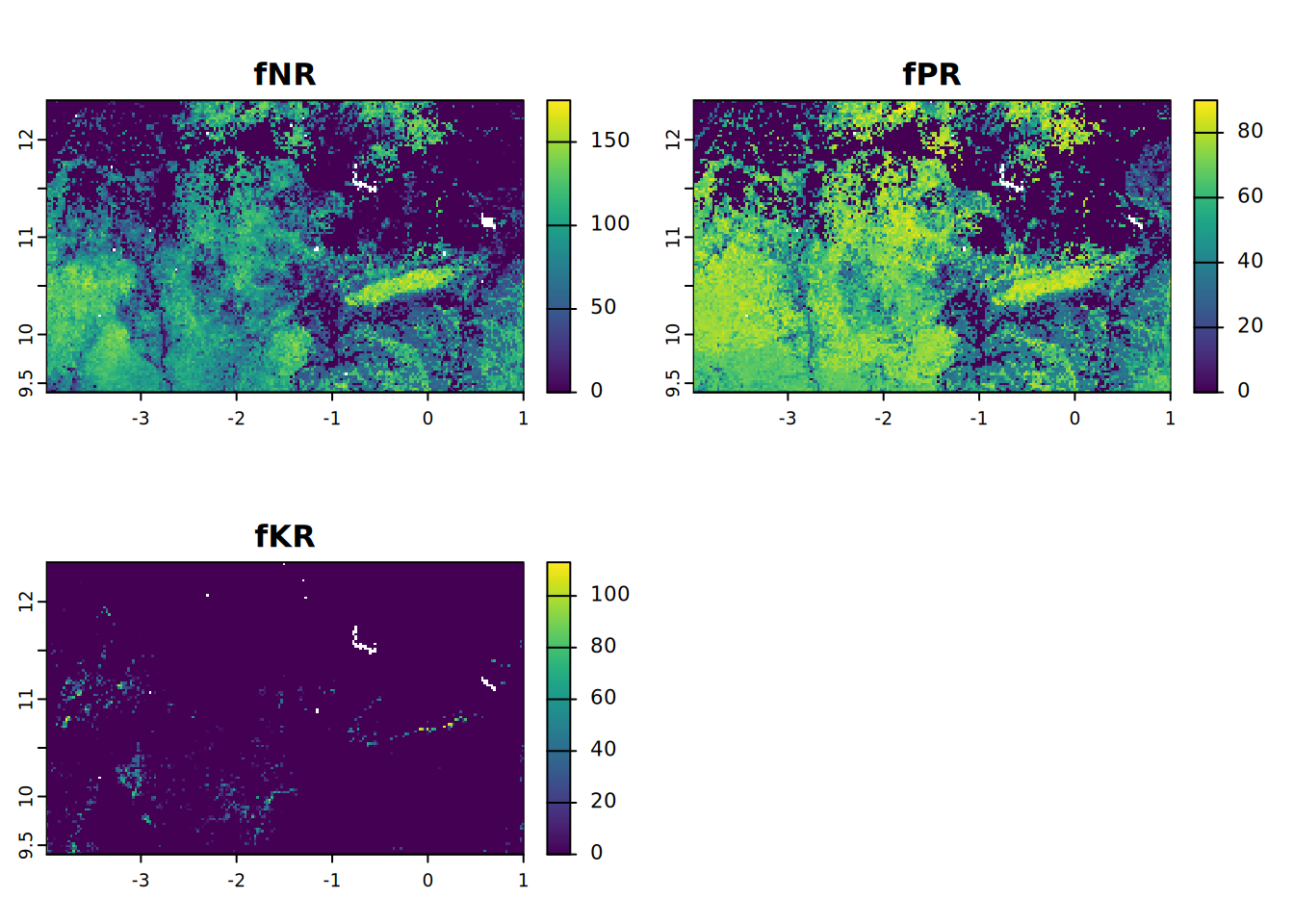
summary <- stats.all(fNPKR)
kable(summary)

## end of script
3.5 Final comments
Above exercise is a simplified version of procedures to assess and map soil qualities as soil water availability and soil nutrient availability and to evaluate those soil qualities relative to crop requirements for formulating agricultural soil management recommendations. The recommended soil management practices aim to enhance the soil qualities to enhance agricultural productivity.
We applied the procedures to soil data read from the Africa SoilGrids.
Thank you.